In this Example, we will learn how to perform single factor ANOVA in Excel 2016.
A single factor ANOVA is used to test the null hypothesis. Which means the mean from all the population are all equal and alternate hypothesis is at least one among the mean is different.
All of the above might be confusing for some people, so let’s gear up & start learning ANOVA single factor in excel with the example.
Here we have marks of Three students in the table.

Select the tab Data > Data Analysis as shown in below screenshot.

Note: can't find the Data Analysis button? Click here to load the Analysis ToolPak add-in.
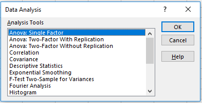
Click on Data Analysis and its dialog box appears.
Now select Anova: Single factor and click OK.

Anova: Single factor dialog box appears. Fill the options as shown below.

Click OK to get the stats for your data.

Conclusion: if the value of F > F crit, we reject the null hypothesis. In this case, 16.59 > 3.40. Therefore, we reject the null hypothesis. The means of the three populations are not all equal. At least one of the means is different.
Hope you got how to test ANOVA single factor tool in Excel 2016. Find more articles on Data Analysis here. Please state your query in the comment box below. We will help you.
Popular Articles:
50 Excel Shortcuts to Increase Your Productivity
How to use the VLOOKUP Function in Excel
The applications/code on this site are distributed as is and without warranties or liability. In no event shall the owner of the copyrights, or the authors of the applications/code be liable for any loss of profit, any problems or any damage resulting from the use or evaluation of the applications/code.
please help me find steps for ANOVA single factor