In this article, we will learn How to Hide gridlines in Excel.
Scenario:
Default features of Excel helps you work on data rather than its formatting. But there comes a time when you no longer require default options. One of the features is show/hide gridlines. Let's understand where to find the switch to turn on (Show) or turn off (Hide) gridlines in excel. The gridlines shown in your excel sheet are very useful, especially when you need to create a template or format a report. But if you do not need them, you can hide these gridlines. Let's understand how to do it as mentioned below.
how to Show/Hide gridlines.
Gridlines in Excel are the horizontal and vertical gray lines that differentiate between cells in a worksheet. The gridlines guide users to differentiate between the cells.
Hide Gridlines :
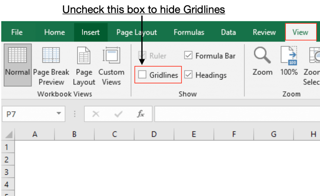
Go to View tab > Uncheck the box which says Gridlines to turn off Gridlines in the workbook
Show Gridlines
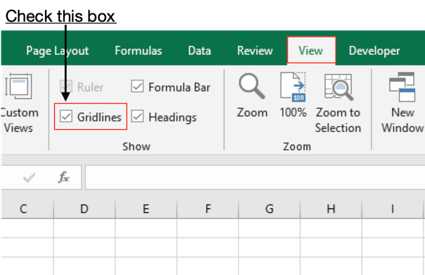
Same as above. Go to View tab > Check the box which says Gridlines to turn on gridlines in the workbook.
Note: You can change the colour of these Gridlines by clicking this link. How to change the colour of gridlines in Excel.
Example :
All of these might be confusing to understand. Let's understand how to use the function using an example. Here we have a sample empty workbook. We need to hide these gridlines as these are going to disrupt the dashboard flow in excel. So Here we follow some steps as mentioned below, which will guide us how to change the default show gridlines in excel.
Follow the steps
First Go to View tab > Uncheck the box adjacent to Gridlines (under Show)

As you can see all the gridlines disappeared from the sheet. Now to switch again to show gridlines follow the same steps as above.
Go to View tab > Check the box adjacent to Gridlines (under Show)

As you can see as you click this box, you get back the gridlines as before.
Here are all the observational notes using the formula in Excel
Notes :
Hope this article about How to Hide gridlines in Excel is explanatory. Find more articles on calculating values and related Excel formulas here. If you liked our blogs, share it with your friends on Facebook. And also you can follow us on Twitter and Facebook. We would love to hear from you, do let us know how we can improve, complement or innovate our work and make it better for you. Write to us at info@exceltip.com.
Related Articles :
How to Select Entire Column and Row Using Keyboard Shortcuts in Excel : Use Ctrl + Space to select whole column and Shift + Space to select whole row using keyboard shortcut in Excel
Excel Shortcut Keys for Merge and Center : This Merge and Center shortcut helps you quickly merge and unmerge cells.
How to use the Shortcut To Toggle Between Absolute and Relative References in Excel : F4 shortcut to convert absolute to relative reference and same shortcut use for vice versa in Excel.
How to use Shortcut Keys for Merge and Center in Excel : Use Alt and then follow h, m and c to Merge and centre cells in Excel.
How to use Shortcut Keys for Sort & filter in Excel : Use Ctrl + Shift + L from keyboard to apply sort and filter on table in Excel.
Paste Special Shortcut in Mac and Windows : In windows, the keyboard shortcut for paste special is Ctrl + Alt + V. Whereas in Mac, use Ctrl + COMMAND + V key combination to open the paste special dialog in Excel.
How to Select Entire Column and Row Using Keyboard Shortcuts in Excel : Selecting cells is a very common function in Excel. Use Ctrl + Space to select columns and Shift + Space to select rows in Excel.
How to Insert Row Shortcut in Excel : Use Ctrl + Shift + = to open the Insert dialog box where you can insert row, column or cells in Excel.
Popular Articles :
50 Excel Shortcuts to Increase Your Productivity : Get faster at your tasks in Excel. These shortcuts will help you increase your work efficiency in Excel.
How to use the VLOOKUP Function in Excel : This is one of the most used and popular functions of excel that is used to lookup value from different ranges and sheets.
How to use the IF Function in Excel : The IF statement in Excel checks the condition and returns a specific value if the condition is TRUE or returns another specific value if FALSE.
How to use the SUMIF Function in Excel : This is another dashboard essential function. This helps you sum up values on specific conditions.
How to use the COUNTIF Function in Excel : Count values with conditions using this amazing function. You don't need to filter your data to count specific values. Countif function is essential to prepare your dashboard.
The applications/code on this site are distributed as is and without warranties or liability. In no event shall the owner of the copyrights, or the authors of the applications/code be liable for any loss of profit, any problems or any damage resulting from the use or evaluation of the applications/code.