Offset Formula in Microsoft Excel

The VLOOKUP, HLOOKUP and INDEX-MATCH are famous and common ways to lookup a values in Excel table. But these are not the only ways to lookup values in Excel. In this article, we will learn how to use the OFFSET function along with the MATCH function in Excel. Yes you read it right, we will use the infamous OFFSET function of Excel to lookup a certain value in a Excel Table.

Generic Formula

Read this carefully:

StartCell: This is the starting cell of lookup Table. Let's say if you want to lookup in range A2:A10, then the StartCell will be A1.

RowLookupValue: This is the lookup value that you want to find in rows below the StartCell.

RowLookupRange: This is the range in which you want to lookup the RowLookupValue. It is the range below StartCell (A2:A10).

ColLookupValue: This is the lookup value that you want to find in columns (headers).

ColLookupRange: This is the range in which you want to lookup the ColLookupValue. It is the range on the right hand side of StartCell (like B1:D1).

So, enough of the theory. Let's get started with an example.

Example: Lookup Sales Using OFFSET and MATCH function From Excel Table

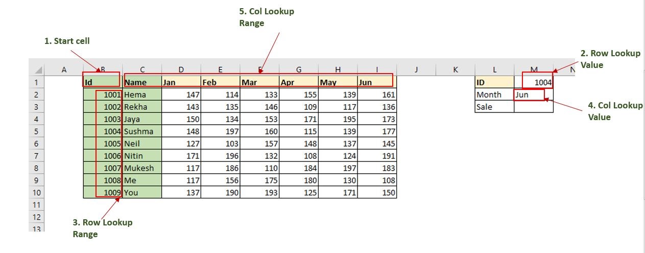
Here we have a sample table of sales done by different employees in different months.

Now our boss is asking us to give the sales done by Id 1004 in the Jun month. There are many ways to do it but since we are learning about the OFFSET-MATCH formula, we will use them to lookup the desired value.

We already have the generic formula above. We just need to identify these variables in this table.

StartCell is B1 here. RowLookupValue is M1. RowLookupRange is B2:B1o (range below the startcell).

ColLookupValue is in M2 cell. ColLookupRange is C1:I1 (Header Range on the right of the StartCell) .

We have identified all the  variables. Let's put them into an Excel Formula.

Write this formula in Cell M3 and hit the enter button.

As you hit the enter button, you get the result promptly.  The sale done ID 1004 in Jun Month is 177.

How does it work?

The OFFSET function's work is to move away from the given starting cell to given row and columns and then return value from that cell. For example, If I write OFFSET(B1,1,1), the OFFSET function will go to cell C2 (1 cell down, 1 cell to right) and returns it value.

Here, We have formula

The first MATCH function returns the index of M1 (1004) in range B2:B10, which is 4. Now the formula is

Next MATCH function returns the index of M2 ('Jun') in range C1:I1, which I7. Now the formula is OFFSET(B1,4,7).

Now the OFFSET function simply moves 4 cells down to the cell B1 which takes it to B5. Then the OFFSET function moves to 7 left to B5, which takes it to I5. That is it. The OFFSET function returns value from cell I5 which 177.

Advantages of this lookup technique?

This is fast. The sole advantage of this method is that it is faster than the other methods. The same thing can be done using the INDEX-MATCH function, or VLOOKUP function. But it is good to know some alternatives. It may come handy some day.

Here are some notes regarding the using the offset formula in Excel.

Notes :

1. OFFSET only returns a reference, no cells are moved.
2. Both rows and cols can be supplied as negative numbers to reverse their normal offset direction - negative cols offset to the left, and negative rows offset above.
3. OFFSET is a "volatile function" – it will recalculate with each worksheet change. Volatile functions can make larger and more complex workbooks run slowly.
4. OFFSET will display the #REF! error value if the offset is outside the edge of the worksheet.
5. When height or width is omitted, the height and width of reference is used.
6. OFFSET can be used with any other function that expects to receive a reference.
7. Excel documentation says height and width can't be negative, but negative values do work.

Hope this article about How to use Offset Formula in Microsoft Excel is explanatory. Find more articles on lookup values and related Excel formulas here. If you liked our blogs, share it with your friends on Facebook. And also you can follow us on Twitter and Facebook. We would love to hear from you, do let us know how we can improve, complement or innovate our work and make it better for you. Write to us at info@exceltip.com.

Related Articles:

Use INDEX and MATCH to Lookup Value : The INDEX-MATCH formula is used to lookup dynamically and precisely a value in given table.  This is an alternative to the VLOOKUP function and it overcomes the shortcomings of the VLOOKUP function.

Sum by OFFSET groups in Rows and Columns : The OFFSET function can be used to sum groups of cells dynamically. These groups can be anywhere in the sheet.

How to Retrieve Every Nth Value in a Range in Excel : Using the OFFSET function of Excel we can retrieve values from alternating rows or columns. This formula takes help of the ROW function to alternate through rows and COLUMN function to alternate in columns.

How to use OFFSET Function in Excel : The OFFSET function is a powerful Excel function that is underrated by many users. But experts know the power of the OFFSET function and how can we use this function to do some magical tasks in Excel formula. Here are the basics of the OFFSET function.

Popular Articles:

50 Excel Shortcuts to Increase Your Productivity : Get faster at your task. These 50 shortcuts will make you work even faster on Excel.

How to use Excel VLOOKUP Function : This is one of the most used and popular functions of excel that is used to lookup value from different ranges and sheets.

How to use the Excel COUNTIF Function : Count values with conditions using this amazing function. You don't need to filter your data to count specific values. The COUNTIF function is essential to prepare your dashboard.

How to use SUMIF Function in Excel : This is another dashboard essential function. This helps you sum up values on specific conditions.