In this article, we will learn Formatting a Value Field in Pivot Tables in Microsoft excel.
Pivot table Scenario:
Pivot table is one of the most powerful tools of Excel. It allows you to quickly summarise a large chunk of organized data. But sometimes the values and fields pivot table created by default is not really required. By default, Excel Pivot table shows sum of numbers if you drag a number column to the value field. You may not want sum but average, or min, or max, etc… In that case you would need to access pivot value field settings.
Example :
All of these might be confusing to understand. Let's understand how to use the function using an example. Here we have a pivot table. Have a look at it.

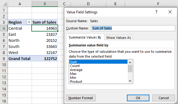
The table shows the summary of data I have. It shows the total sales done by each region. But instead of total sales, I want to get the average sales. For that I will need to access values field settings.
To access Value Fields Settings, right click on any value field in the pivot table. A list of options will be displayed. In the end of the list (most 3rd from last) you will see value field settings. Click on it and a dialog box will appear.


Another way to access value field settings is the area where we drop fields for the pivot table.
You can go to the values area. Click on the small arrow head. As the last option, you will see Value Fields Settings.

You can also use the Pivot Table Analyze menu from Ribbon to access value field settings. It is the second option in the Pivot Table Analyze menu. Just make sure that you have a value field selected.

Now that you have accessed the value fields settings, you can modify the field using the available options. For our example, we needed the average of sales done by each region. So we change the summarize value fields by to Average. You can also change the name of the field here.

You can see one more tab here that is "Show Value As". Here you can choose to show value as percentage of total or difference between two columns, rank etc.
The Field Settings allows you to modify the structure of the table. The Field settings can be accessed by right clicking on any row or column heading or subheading.

Another way is the dropping area of fields. Same as the value field settings, you can click on the little arrow head on the rows, or columns section to open the field settings.

And another way to access the field settings is the pivot table analyze tab of ribbon, same as the value fields settings.
From field settings of pivot tables, you modify the subtotals of the pivot table, change the layout and print settings. You can choose to show items in tabular format or not, choose to repeat item labels or not. Choose to insert a blank line after each item label or not. Choose to show items with no data or not.

Hope this article about Formatting a Value Field in Pivot Tables in Microsoft excel is explanatory. Find more articles on calculating values and related Excel formulas here. If you liked our blogs, share it with your friends on Facebook. And also you can follow us on Twitter and Facebook. We would love to hear from you, do let us know how we can improve, complement or innovate our work and make it better for you. Write to us at info@exceltip.com.
Related Articles :
Excel Pivot Tables | Pivot tables are one of the most powerful tools and one who knows all the features of pivot tables can increase his productivity exponentially. In this article we will learn all about pivot tables in detail.
How to use the Dynamic Pivot Table in Excel | To create a dynamic pivot table we use named ranges and tables in excel. But that is not all. A dynamic pivot table will reduce work of data maintenance and it will consider all newly added data as the source data.
How to Refresh Pivot Charts | To refresh a pivot table we have a simple button of refresh pivot table in the ribbon. Or you can right click on the pivot table. Here's how you do it.
Conditional Formatting for Pivot Table | Conditional formatting in pivot tables is the same as the conditional formatting on normal data. But you need to be careful while conditional formatting pivot tables as the data changes dynamically.
How to get subtotal grouped by date using GETPIVOTDATA function in Excel | This is a special function that is specially used to work with data of pivot tables. It is used to retrieve values from pivot tables using the table columns and rows headers.
Popular Articles :
How to use the IF Function in Excel : The IF statement in Excel checks the condition and returns a specific value if the condition is TRUE or returns another specific value if FALSE.
How to use the VLOOKUP Function in Excel : This is one of the most used and popular functions of excel that is used to lookup value from different ranges and sheets.
How to use the SUMIF Function in Excel : This is another dashboard essential function. This helps you sum up values on specific conditions.
How to use the COUNTIF Function in Excel : Count values with conditions using this amazing function. You don't need to filter your data to count specific values. Countif function is essential to prepare your dashboard.
The applications/code on this site are distributed as is and without warranties or liability. In no event shall the owner of the copyrights, or the authors of the applications/code be liable for any loss of profit, any problems or any damage resulting from the use or evaluation of the applications/code.