In this article, we will compare two columns using the Conditional Formatting tool in Excel 2016.
It would be difficult to see various trends just for examining your Excel worksheet. Conditional Formatting provides a way to visualize data and make worksheets easier to understand. It allows you to apply formatting basis on the cell values such as colours, icons and data bars. For this, we will create a rule in Conditional Formatting.
Let’s understand how to compare two columns in excel taking the below example.
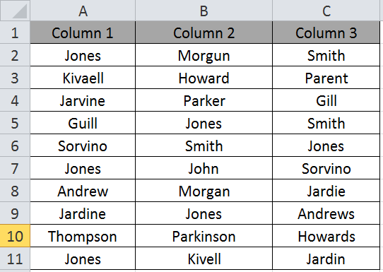
Here we have a list of names in all three columns. We need to find out the repeated or duplicate names.
So for this, we are going to use Conditional formatting.

Select the cells you need to apply conditional formatting.
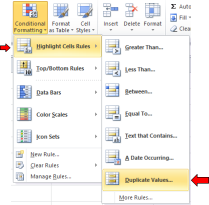
Click Home > Conditional Formatting > Highlight Cell Rules > Duplicate values

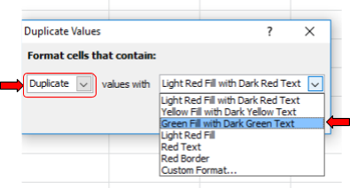
A dialog box appears

Select the Duplicate option from the dropdown list as shown in above snapshot. Select the type of format and click OK.
You can find duplicate values are highlighted with Green fill with Dark Green Text as shown below.

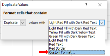
You can customize your highlight Index and formatting for your data by clicking on the Custom Format option as shown below.

You can compare two columns in excel for differences using Conditional Formatting in Excel. Please do check out other articles on Conditional Formatting. Please state your queries regarding Conditional formatting down in the comment box. We will help you.
Related Articles:
How to Compare Two Strings in Excel
Using If Function to Compare Dates of Two Cells
Popular Articles:
50 Excel Shortcut to Increase Your Productivity
How to use the VLOOKUP Function in Excel
How to use the COUNTIF function in Excel 2016
How to use the SUMIF Function in Excel
The applications/code on this site are distributed as is and without warranties or liability. In no event shall the owner of the copyrights, or the authors of the applications/code be liable for any loss of profit, any problems or any damage resulting from the use or evaluation of the applications/code.