Dynamic charts using camera tool in Microsoft Excel 2010

In this article, we will learn how to make a dynamic chart using the camera tool in Microsoft Excel 2010.

The camera tool is used for taking the snapshot of the range and can display it from one workbook to another workbook wherever we want to display and the snapshot image is updated dynamically so when we change the data, snapshot will get changed automatically. Also, this tool is used for providing the effects to range as picture.

Before using the Camera tool, it has to be added in the toolbar of menu.

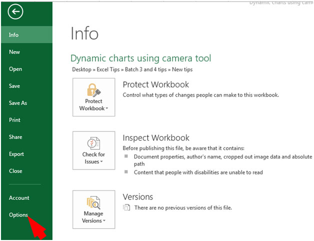
Go to File Tab in the ribbons.

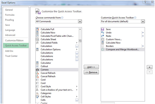
Select option, and then choose the option of the Quick Access Toolbar.

Select all commands from the drop down list of Choose commands.

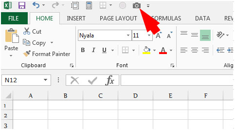
Find camera tool select, click on add and press OK.
Camera tool will display in the top of Menu bar.

Let’s take an example & understand how we can use the camera tool for dynamic chart.

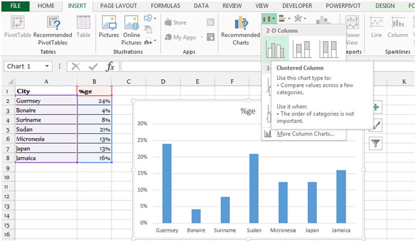
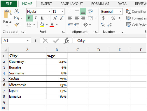
We have data from A1 to B8.

How to prepare a regular chart?

Select the range of data.
Go to insert tab, and Select Column Chart from the group of chart.

Change the alignment of text, select the area of city, and then with right click of the mouse, select format chart area. The dialog box will appear.

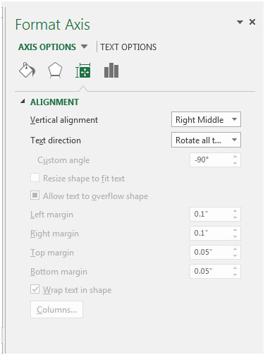
Select alignment tab and change the text direction from the drop down list.
Select rotate all text 270 degree.

Select the cells surrounding of the chart, and click on the camera tool and click anywhere in the worksheet. The chart will be created with the Dynamic picture link of the cells.

The green rotate control on the top of picture is showing. We can rotate it and excel places snapshot of the range we have selected.
Drag the object to the right to rotate the excel chart. Drop the rotate control at 90 degree to create the vertical chart.

When we click on the snapshot, the format tool gets appeared in the Menu bar.

There are so many options available to make it presentable.
We can crop the snapshot.

Select the snapshot, go to the format tool bar, and then click on crop and adjust it till the chart area.

Note: This is dynamic picture of the range. When the original chart will change, the picture will keep up and change also.

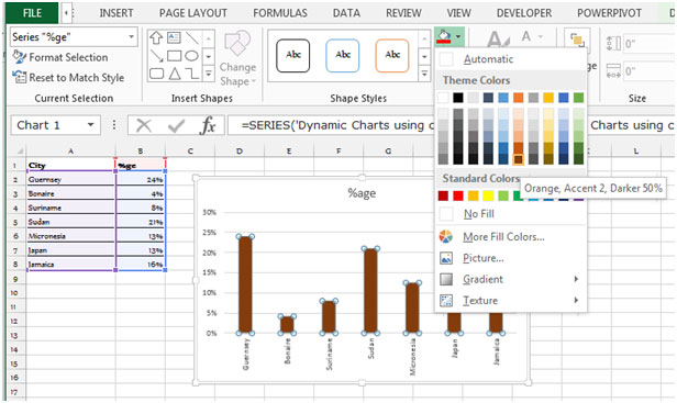
Let’s understand with an example: Select the columns of original chart and change the color.

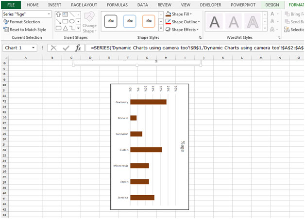
The color of columns gets changed in dynamic chart too.

This is all about the Dynamic charts using camera tool inMicrosoft Excel in 2010 & 2013.

Jon Peltier
December 13, 2014 at 4:01 pm

The camera tool places an enormous drain on Excel resources. If you have more than about half a dozen on a sheet, they will just bog Excel right down.

What is the benefit of creating a column chart and rotating a picture of it, rather than creating a bar chart?

And if you just want a picture of the same chart, unrotated, it's better to simply copy and paste the original chart.

Reply ↓