In this article we will learn how we can retrieve the player who scored the highest number of points in Microsoft Excel 2010.
To retrieve the name of the player who scored the highest number of points, we will use a combination of INDEX, MATCH & MAX functions to get the output.
INDEX: Returns a value or reference of the cell at the intersection of a particular row and column, in a given range.
Syntax: =INDEX(array,row_num,column_num)
MATCH function searches for a specified item in a selected range of cells, and then returns the relative position of that item in the range.
Syntax =MATCH(lookup_value,lookup_array,match_type)
MAX: Returns the maximum number from a range of cells or array. For example,if a list of numbers contains 5, 6, 7, 8, 9 & 10, then the output will be 10.
Syntax =MAX(number1,number2,...)
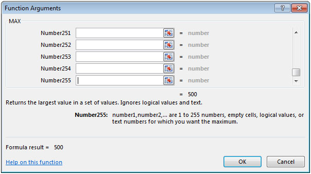
There can be maximum 255 arguments. Refer below shown screenshot:

Let us take an example:
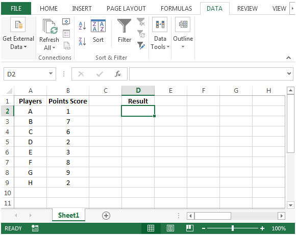
We have number of players in column A & the points scored by them in column B. We need a formula to determine which player has scored the highest points.


In this way, if we have a similar requirement, then we can achieve it by using INDEX, MATCH & MAX functions together.
The applications/code on this site are distributed as is and without warranties or liability. In no event shall the owner of the copyrights, or the authors of the applications/code be liable for any loss of profit, any problems or any damage resulting from the use or evaluation of the applications/code.
You can do this using Vlookup function with Max function.It is easy. But you will have to re-arrange the table Points first and names second.
=Vlookup(Max(range),table_array,column number,0)
Nice Prav.
This will work too.
Please someone helps me for below issue... I got error when writing formula for max high score more than one person..
AAA 10
BBB 20
CCC 30
DDD 25
EEE 30
{=INDEX($A$1:$A$5,SMALL(IF($B$1:$B$5=MAX($B$1:$B$5),ROW($B$1:$B$5)-1),ROW(B1)-1))}
What do I do if I have duplicates as the highest value?
Ex : A1 and A15 have same highest score. I want to show both names and score together. Even I used below formula, still facing error and showed mistake results.
=INDEX($A$1:$A$15,SMALL(IF($B$1:$B$15=MAX($B$1:$B$15),ROW($B$1:$B$15)-1),ROW(B1)-1))
What do I need to fix my formula to get correct result?
What if I want to add subject, For example, I want to know who toped in English and who in science etc.
please help.
In this case, we have criteria like countifs, right? Here, I have explained how to use MAX with conditions in Excel 2016 or older:
https://www.exceltip.com/statistical-formulas/calculate-max-if-condition-match.html
If you have Excel 2019 or 365 then you can use MAXIFS function:
https://www.exceltip.com/excel-365-functions/the-excel-maxifs-function.html
I would like the first name and the surname (family name) and then the highest score. First name and surname in different but adjoing cells
Hi.,
Thanks fro posting this. How about if there are criterias that need to be satisfied in getting the name who got the highest score? For example, i want to get the name of the student who got the highest score in engineering department for all freshman only? What will be the formula?
Works excellently
How would I do this with a criteria?
E.g. Players is still the value I'm wanting to return, but based on an additional column specifying Gender... So I would want to find the highest scoring player for a Boy and the highest scoring player for a Girl?
Hi,
Thanks for the tip. Quick question-
What do I do if I have duplicates as the highest value. For ex. in your example, lets say player H also had 9 points.
What do I do in case I need to get both the highest player names?
Thanks
Hi Kerishma,
You can use below array formula to find both the highest player names. Paste below formula in cell D2 and press F2 and then press Ctrl + Shift + Enter. Cell D2 will give first highest player name. To get second highest player name, drag the formula in cell D2 to D3, it will give second highest player name.
=INDEX($A$2:$A$9,SMALL(IF($B$2:$B$9=MAX($B$2:$B$9),ROW($B$2:$B$9)-1),ROW(B2)-1))
=INDEX($A$2:$A$9,SMALL(IF($B$2:$B$9=MAX($B$2:$B$9),ROW($B$2:$B$9)-1),ROW(B2)-1))
if use this formula i am getting two names which are having same value. but next names in order are not coming
This is a good one.
Hi! Thanks for posting this! I was wondering if two players have the highest amount of points what would be needed in the formula to display both names?
I too would like to know the same, if there is a tie, how can you display both names of the winners or more if there is multiple winners?
The Formula is: =INDEX($A$2:$A$6,MATCH(LARGE($C$2:$C$6,E2),$C$2:$C$6,0))
Hi Matt and Evan!. If two players have same score and you want to know the name of both of them, you gonna need a helping column.
In below data, column A has names, and column B has scores. Now here is the trick. in column c you gonna have a formula (=rand()+B1 and so on).
Name Score Helper
Riya 50 =RAND()+B2
Ramesh 50 =RAND()+B3
Raghav 35 =RAND()+B4
Raju 50 =RAND()+B5
Rahul 20 =RAND()+B6
Now wherever You want to get your top scorers, prepare this table. I did in E and F column. E has the sr no. very important. then our formula to retrieve all top scorers.
Sr.No. Name
1 Raju
2 Ramesh
3 Riya
Formul written in F1 and F2 and F3 is. Not explaining it here but will prepare a explanation article for you guys.
Top Scores Name
1 =INDEX($A$2:$A$6,MATCH(LARGE($C$2:$C$6,E2),$C$2:$C$6,0))
2 =INDEX($A$2:$A$6,MATCH(LARGE($C$2:$C$6,E3),$C$2:$C$6,0))
3 =INDEX($A$2:$A$6,MATCH(LARGE($C$2:$C$6,E4),$C$2:$C$6,0))
this will not only give you the tie values but all top values. either it be duplicate or non. just enter the serial numbers and drag down the formula.
But if you want to get only clashing values than use below array formula.
{=INDEX($A$2:$A$9,SMALL(IF($B$2:$B$9=MAX($B$2:$B$9),ROW($B$2:$B$9)-1),ROW(B2)-1))}
use control+ shift+ enter key after writing this formula. Drag it down in below cells. all clashing values will be fetched.