Retrieving the Last Value and the Last Character in a Row in Microsoft Excel 2010

To retrieve the last value, we use a combination of “INDEX”, “MAX”, and “COLUMN” functions, and to retrieve the last character in a row, we use the “HLOOKUP” and “REPT” functions in Microsoft Excel 2010.

INDEX: The Index formula returns a value from the intersection between the row number and the column number in an Array. There are 2 syntaxes for the “INDEX” function.

1st Syntax of “INDEX” function:=INDEX (array, row_num, [column_num])

2nd Syntax of “INDEX” function:=INDEX (reference, row_num, [column_num], [area_num])

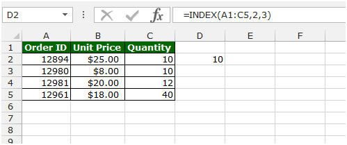
For example:- We have data in range A1:C5 in which column A contains Order Id, column B contains Unit Price, and column C contains Quantity.

Follow below given steps:-

• Write the formula in cell D2.
• =INDEX(A1:C5,2,3)
• Press Enter on your keyboard.
• The function will return 10, which means 10 is available in 2^nd row and 3^rd column.

 

 
MAX: This function is used to return the largest number in a set of values. It ignores logical values and text.

Syntax of “MAX” function:            =MAX(number1, [number2],….)

Example: Range A1:A4 contains numbers, and we need to return the maximum number from this range.  

Follow the below given steps:-

• Select the cell B1 and write the formula.
• =MAX(A1:A4)
• Press Enter on your keyboard.
• The function will return 9.
• 9 is the maximum value in the range A1:A4. 

 

 
COLUMN: This function is used to return the column number of a reference.

Syntax of “COLUMN” function:     =COLUMN(reference)

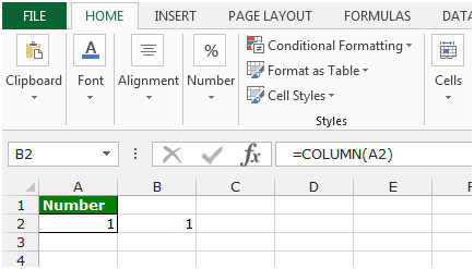
For Example: If we want to return the column number for the cell A1, we need to follow below given steps:-

• Write the formula in cell B2.
• =COLUMN(A2)
• Press Enter on your keyboard.
• The function will return 1, which means this is column 1.

 

 
HLOOKUP: The function is used for looking a value in the top row of a table or array of values and returns the value in the same column from a row you specify.

Syntax of “HLOOKUP” function:            =HLOOKUP(lookup_value,table_array,row_index_num,[range_lookup])

Uses of Hlookup Function

We use this function to pick the values from one data to another, but to meet the condition we should have the common values in both data sets so that we can easily pick the value.

Let’s take an example and understand how and where we can use Vlookup function in Microsoft Excel 2010.

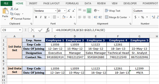
Example 1: We have 2 data sets in which we require joining date from 1^st data to 2^nd data.

 

 
To pick the value from 1^st data to 2^nd data, the common value we have is Emp. Code. So we will put the Hlookup function through Emp. Code. We need to follow below mentioned steps to pick the joining date:-

• Select the cell C9 and write the formula.
• =HLOOKUP(C8,$C$2:$G$3,2,false)
• Press Enter on your keyboard.
• The function will return the joining date for this L1056 Emp code.
• To return the date of joining to all the employees, copy the same formula and paste in the range D9:G9.

 

 
Note: If the common value we do not have in other data from which we want to pick the data, then the formula will give the #N/A error. As you can see in above snapshot, the employee code L1089 in not available in 1st data set so formula is giving the error.

REPT:- This function is used to repeat text a given number of times. Use REPT to fill a cell with a number of instances of text string.

Syntax of “REPT” function:           =COLUMN(reference)

For example:- Write the formula in cell A1 =REPT("a",10), and press Enter on your keyboard. The function will show that “a” is repeating 10 times.
 

 
MODE: This function is available for compatibility with Excel 2007 and earlier. It returns the most frequently occurring or repetitive value in an array or range of data.

Syntax of “MODE” function:          =MODE(number1, [number2],……..)

For Example:-We have number list in the range A1:A5.

To return the mode of numbers, follow below given steps:-

• Write the formula in cell B1.
• =MODE(A1:A5)
• Press Enter on your keyboard.
• The function will return 1.

 

 
IF: - Check whether a condition is met and returns one value if True and another value if False.

The syntax of “IF” function =if(logical test,[value_if_true],[value_if_false])

Firstly, the formula will do the logical test to know if the output of logical test is true or false.

For example:Cell A2 and A3 contain the number 3 and 5. If the number is 3, the formula should display “Yes”, else “No”.

=IF (A1=3,"Yes","No")
 

 
Let’s take an example to understand how we can retrieve the last value and the last character in a row.

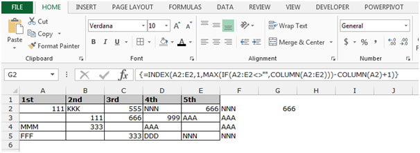
We have data in range A2:E5 in which cells contain characters and numbers individually. Some of the cells in the range may be empty.

We want to retrieve both the last values (of any type) and the last character that appears in each row of the range.

 

 
To find the last character for each row, follow below given steps:-

• Write the formula in cell F2.
• =HLOOKUP(REPT("z",10),A2:E2,1)
• Press Enter on your keyboard.
• The function will return the last character for each row.

• Copy the same formula by pressing the key Ctrl+C and paste in the range F3:F5 by pressing the key Ctrl+V on your keyboard.

 

 
To find the last value (of any type) in each row, follow below given steps:-

• Write the formula in cell G2.
• =INDEX(A2:E2,1,MAX(IF(A2:E2<>"",COLUMN(A2:E2)))-COLUMN(A2)+1)
• Press Shift+Ctrl+Enter on your keyboard.
• {=INDEX(A2:E2,1,MAX(IF(A2:E2<>"",COLUMN(A2:E2)))-COLUMN(A2)+1)}

• The function will return the last character for each row.

• Copy the same formula by pressing the key Ctrl+C and paste in the range G3:G5 by pressing the key Ctrl+V on your keyboard.