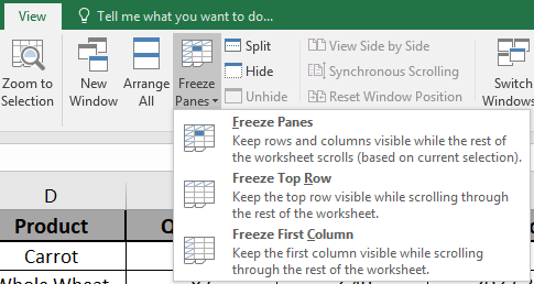
In this article, we will learn How to Freeze Panes in Microsoft Excel.
Freeze panes: - We use this option to freeze a portion of sheet to keep it visible while you scroll through the rest of the sheet. This is useful for checking out data in other parts of your worksheet without losing your headers or labels.
Shortcut key of Freeze panes: - Alt+W,F,F
When you have a huge amount of data under a common heading you are unable to see the heading when scrolled down the worksheet. What freeze panes does is it lets you freeze particular rows and columns of your choice so that you can see that frozen portion even when the rest of the datas are being scrolled. It makes your job much easier when you have thousands of data under one heading. Freezing and unfreezing panes changes the view of the data without changing the data itself.
Example :
All of these might be confusing to understand. Let's understand how to use the function using an example.
Here we have an example of multiple columns & rows to make the article more understandable.

Go to View > Freeze panes

Select the type, you wish to freeze.
Here We wish to Freeze Top Row
Select Freeze top row from Freeze panes drop down options

As you can see 1st Row is Freezed as the second row its showing is 20. Scrolling more down the page first row will help you track the label field.
Freeze panes let you view your large data without any keeping track of Row or Column label.
What if you want to select more than one row or column or freeze something to the right side?
There is solution to that too first of all you will notice a little bar on top of the vertical scroll bar when you place your mouse there you will see that your mouse pointer has become a two headed arrow now left click the mouse button and drag down underneath the row you want to freeze and go to freeze panes option from the view tab and click it.
Similarly there is a small bar on the right side of the horizontal scroll bar, placing your mouse pointer on it will show a similar two headed arrow effect now click your mouse and drag it up to the column you want to freeze and click on the freeze panes option to freeze the column.
Notes:
You cannot freeze or unfreeze panes while you are in cell editing mode or page layout view.
You cannot freeze or unfreeze if the worksheet is protected.
Don’t select the A1cell as it is not possible to select rows or columns above the A1 cell. Excel will freeze the panes near the center of the work space instead.
When you print the worksheet you will not get what you have seen after freezing, you will only get the regular worksheet.
Hope this article about How to Freeze Panes in Microsoft Excel is explanatory. Find more articles on calculating values and related Excel formulas here. If you liked our blogs, share it with your friends on Facebook. And also you can follow us on Twitter and Facebook. We would love to hear from you, do let us know how we can improve, complement or innovate our work and make it better for you. Write to us at info@exceltip.com.
Related Articles :
How to use the Shortcut To Toggle Between Absolute and Relative References in Excel : F4 shortcut to convert absolute to relative reference and same shortcut use for vice versa in Excel.
How to use Shortcut Keys for Merge and Center in Excel : Use Alt and then follow h, m and c to Merge and centre cells in Excel.
How to Select Entire Column and Row Using Keyboard Shortcuts in Excel : Use Ctrl + Space to select whole column and Shift + Space to select whole row using keyboard shortcut in Excel
Paste Special Shortcut in Mac and Windows : In windows, the keyboard shortcut for paste special is Ctrl + Alt + V. Whereas in Mac, use Ctrl + COMMAND + V key combination to open the paste special dialog in Excel.
How to Insert Row Shortcut in Excel : Use Ctrl + Shift + = to open the Insert dialog box where you can insert row, column or cells in Excel.
50 Excel Shortcuts to Increase Your Productivity : Get faster at your tasks in Excel. These shortcuts will help you increase your work efficiency in Excel.
Popular Articles :
How to use the IF Function in Excel : The IF statement in Excel checks the condition and returns a specific value if the condition is TRUE or returns another specific value if FALSE.
How to use the VLOOKUP Function in Excel : This is one of the most used and popular functions of excel that is used to lookup value from different ranges and sheets.
How to Use SUMIF Function in Excel : This is another dashboard essential function. This helps you sum up values on specific conditions.
How to use the COUNTIF Function in Excel : Count values with conditions using this amazing function. You don't need to filter your data to count specific values. Countif function is essential to prepare your dashboard.
The applications/code on this site are distributed as is and without warranties or liability. In no event shall the owner of the copyrights, or the authors of the applications/code be liable for any loss of profit, any problems or any damage resulting from the use or evaluation of the applications/code.
This was very helpful, I was use to the old way now I know the new way. This helps with long files with the same information running on.