In this article, we will learn How to use the ADDRESS function in Excel.
Text manipulation in Excel
While working on Excel, sometimes some information is combined into one. For example Employee ID of any employee is unique, but has all the information like department name, joining year and some initials of the name. These informations are usually located using a special character. Like if you need to find the person names used in all the employee email id. So you know a pattern something like abc@gef.co. just extract the values left of @ in the value.
LEFT Function in Excel
LEFT: Returns the specified number of characters starting from the left-most character in the text string.
LEFT Function syntax:
| LEFT (text,[num_chars]) |
text : text to extract from
[num_chars] : number of characters from the left of text
Example :
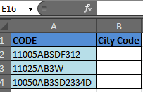
All of these might be confusing to understand. Let's understand how to use the function using an example. Here In this example Cell A2 contains a code whose first 5 characters are city code, to separate the city code from the text, we will use:

| =LEFT(A2, 5) |
Thus, the function will return “11005”, as shown in the image. Copy the formula in the cells below to do the same for other codes.

This formula is the command that locates and selects specific text.
Let’s take an example to understand how to select the first 5 characters from another cell.
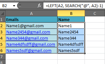
Example 1: I have a list of email addresses in column A. The username is the first 5 characters of the email addresses.

To separate the first 5 characters from the list, follow the below mentioned steps:-
Select Cell B2, write the formula
| =LEFT (A2, 5) |
and press Enter on the keyboard.
The function will return the first 5 characters from the cell.
To copy the formula in all cells select cell B2, press the keys“CTRL + C” on the keyboard and select the range B3 to B6 and press key “CTRL + V”.

Note: If there is no specific number of characters for the name in the email id, you can use the “Left” function along with the “Search” function.

SEARCH: The SEARCH function return the starting position of a text string which it locates from within the specified text string.
Syntax of “SEARCH” function:
| =SEARCH (find_text,within_text,[start_num]) |
Note: SEARCH is case sensitive in excel. It means if “a” and “A” is different for this excel function.
| Use FIND instead of SEARCH if you don’t want it to be case sensitive. |
Example:
Cell A1 contains the text “Bush, George”
=SEARCH (“,”, A1, 1), the function will return 5.

This means that the “comma” is located at the 5 positions in the text string, starting from the left-most character.
To separate the name from the list by using the “Left” function along with “Search” function follow the below mentioned steps:-
Select the Cell B2, write the formula. Press Enter on the keyboard.
| =LEFT (A2, SEARCH (“@”, A2)-1). |

The function will return the name from the email id.
Copy the formula in all cells press key “CTRL + C” on the keyboard and select the range B3 to B6 and press key “CTRL + V
Extract Text From A String In Excel Using Excel’s LEFT And RIGHT Function
Data cleaning in excel is easy. Here I am going to explain how you can extract specific text in excel 2016 from a cell and leave behind garbage data.

In the above image, I am provided with data in Excel. It has Name, Age, and if the person has any insurance or no (Y/N). To use this data, I need to extract data in different columns. Each column should contain only one kind of value. Once it’s done we can make pivot reports in excel that will tell us better about the data. So let's get started.
Excel RIGHT Function to Extract Data From Right of The Text
Let’s start with the easiest one. In this example, we have “Has insurance?” data at the end of the string. And that is only one character (Y or N). To extract this data we will use the RIGHT Formula Excel provides. The RIGHT function is available in Excel 2016, Excel 2013, Excel 2010 and older versions of Excel.

RIGHT function in excel takes only two arguments. First the TEXT, and second the NUMBER OF CHARACTERS you want to extract from the right in excel.
Generic Formula:
| =RIGHT(text, number_of_Characters) |
Here, we have our text in cell B3 and the number of characters we want to extract is 1. Just write this formula in excel in cell D3 or wherever you want to have this data.
| =RIGHT(B3,1) |
You will have your result in cell D3. just copy or drag down this formula in the cells below.
Excel LEFT Function to Extract Data From Left of The Text
Now let's get our age. Before explaining, let me show you the formula. Copy this formula in desired cells.
| =LEFT(RIGHT(B3,4),2) |
In the above formula, we have combined LEFT and RIGHT functions to get our specific text from the string. This is how it looks.

Now let's understand this puny formula.
Every function works from inwards to outwards. So let's start with:
RIGHT(B3,4): It simply extracts 4 characters from a given text. That gives us 30_Y. Why 4? Since we know that age is only one of two characters, and we have 1 “_” and 1 Y or N.
LEFT(RIGHT(B3,4),2): Now we have our text that starts with age that is of 2 characters. Here comes the LEFT function into action. It takes RIGHT(B3,4) as its text argument and extracts 2 characters from that. That gives us 30 for the first cell. Copy the formula in the cells below and you will get the rest of the data as shown in the image above.
Generic Formula for LEFT:
| =LEFT(text, Number_of Characters) |
Just like the RIGHT function in excel LEFT function of Excel also takes two same arguments. It just extracts data from the left of the string provided.
Excel LEFT and Right Function to Extract unknown length of Text from a String
Just paste this formula in desired cells to extract the name from the text in excel.
| =LEFT(B3,LEN(B3)-5) |

In the above examples, we knew the exact number of texts to extract from the given text. But now, we don’t know how lengthy a name is. What can be done?
We do know that the name is followed by exact 5 characters. 1 for space, 2 for the age, 1 for “_” underscore, and one for the Y.
If we can get all number of text and then subtract 5 from that then we will have the exact number of text for the name.
For finding the length of a text in Excel we can use the LEN function. The LEN function of excel returns the number of characters involved.
Syntax:
| =LEN(text) |
So LEN(B3) returns 20.
LEN(B3)-5 returns 15. And this the length of the name in cell B3
At last LEFT(B3, LEN(B3)-5) gives us Georgina Schalk as a result. When you copy the formula in the cells below, you get all the names.
Now you can prepare reports like this based on extracted data using pivot tables. It tells us that half of our subjects have insurance and the other half don’t.

LEFT and RIGHT FUNCTION of excel is very powerful and useful for data cleaning. When combined with LEN function, FIND function and SUBSTITUTE function of excel they can extract any substring within a string in excel.
Video: How to use LEFT function in Microsoft Excel
Watch the steps in this short video, and the written instructions are above the video
Here are all the observational notes using the LEFT function in Excel
Notes :
Hope this article about How to use the LEFT function in Excel is explanatory. Find more articles on calculating values and related Excel formulas here. If you liked our blogs, share it with your friends on Facebook. And also you can follow us on Twitter and Facebook. We would love to hear from you, do let us know how we can improve, complement or innovate our work and make it better for you. Write to us at info@exceltip.com.
Related Articles :
How to use the RIGHT function in Excel : Extract text from the RIGHT of the text just like the left function explained above in excel. Learn RIGHT function syntax and usage with an example
How to use the MID function in Excel : Extract text from the middle of the text just like the left or right function in excel. Learn MID function syntax and usage with an example
How to use the FIND function in Excel : find known text in the given cell and return the position of known text like the function usage explained above in excel. Learn FIND function syntax and usage with an example
How to use the SEARCH function in Excel : locate known text in the given cell and return the position of known text like the function usage explained above in excel. Learn SEARCh function syntax and usage with an example
Extract Text From A String In Excel Using Excel’s LEFT And RIGHT Function
How to Use TRIM function in Excel: The TRIM function is used to trim strings and clean any trailing or leading spaces from string. This helps us in the cleaning process of data a lot.
How to use the CLEAN function in Excel: Clean function is used to clean up unprintable characters from the string. This function is mostly used with the TRIM function to clean up imported foreign data.
Replace text from end of a string starting from variable position: To replace text from the end of the string, we use the REPLACE function. The REPLACE function uses the position of text in the string to replace.
How to Check if a cell contains one of many texts in Excel: To find check if a string contains any of multiple text, we use this formula. We use the SUM function to sum up all the matches and then perform a logic to check if the string contains any of the multiple strings.
Count Cells that contain specific text: A simple COUNTIF function will do the magic. To count the number of multiple cells that contain a given string we use the wildcard operator with the COUNTIF function.
Excel REPLACE vs SUBSTITUTE function: The REPLACE and SUBSTITUTE functions are the most misunderstood functions. To find and replace a given text we use the SUBSTITUTE function. Where REPLACE is used to replace a number of characters in string…
Popular Articles :
How to use the IF Function in Excel : The IF statement in Excel checks the condition and returns a specific value if the condition is TRUE or returns another specific value if FALSE.
How to use the VLOOKUP Function in Excel : This is one of the most used and popular functions of excel that is used to lookup value from different ranges and sheets.
How to use the SUMIF Function in Excel : This is another dashboard essential function. This helps you sum up values on specific conditions.
How to use the COUNTIF Function in Excel : Count values with conditions using this amazing function. You don't need to filter your data to count specific values. Countif function is essential to prepare your dashboard.
The applications/code on this site are distributed as is and without warranties or liability. In no event shall the owner of the copyrights, or the authors of the applications/code be liable for any loss of profit, any problems or any damage resulting from the use or evaluation of the applications/code.