The GETPIVOTDATA function extracts the data stored in a PivotTable report. You can use this function to retrieve data as long as it is visible in the pivot table.
The easiest way to understand how the Getpivotdata function works:
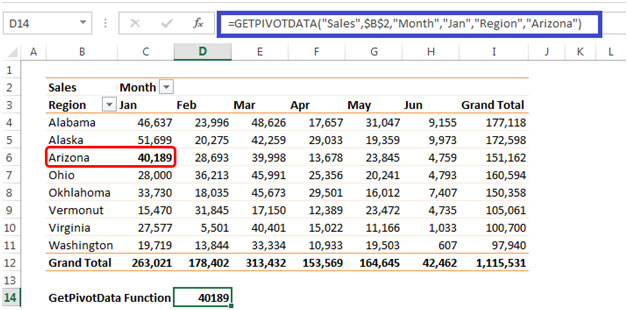
To extract data from a cell in a pivot table, we can enter a normal cell link in cell D14, for example=C6.The GetPivotData function will automatically generate the formula as shown in the below screenshot:

Syntax =GETPIVOTDATA(data_field,pivot_table,field,item,...)
Let’s understandarguments of this
formula=GETPIVOTDATA("Sales",$B$2,"Month","Jan","Region","Arizona")
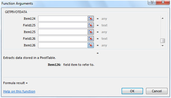
Field & Items are entered as a pair & we can use a maximum as 126Arguments as shown in the below picture.

Using Cell References in GetPivotData
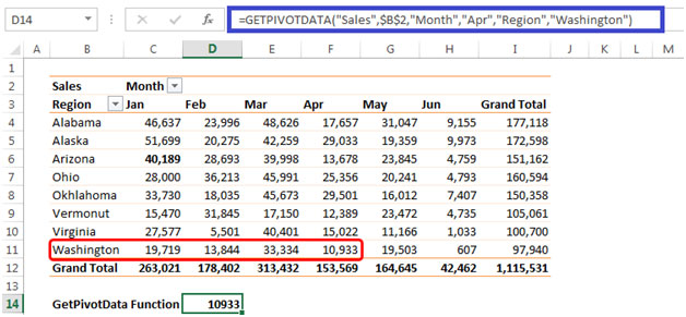
In a GetPivotData formula, refer to the pivot table, and the field(s) and item(s) that you want the data for. For example, this formula gets the Total, from the pivot table in D14, for the Month field, and the Washington item.

To make a GetPivotData formula more flexible, we can refer to worksheet cells, instead of typing the item or field names in the arguments.
Using the same example, we can enter “Apr” in cell L4 & “Washington” in cell L5. Then, change the formula in cell D14to reflect L4 & L5, instead of typing “Apr” & "Washington" in the formula.

Formula in cell D14 =GETPIVOTDATA("Sales",$B$2,"Month",L4,"Region",L5)
If you do not want to automatically generate the GetPivotData Function you can get rid of it by following the given steps:


Alternatively, Under File?Options?Click on Formulas de-select Use GetPivotData functions for PivotTable references. Click on Ok.

In this way we can extract data from pivot table.
The applications/code on this site are distributed as is and without warranties or liability. In no event shall the owner of the copyrights, or the authors of the applications/code be liable for any loss of profit, any problems or any damage resulting from the use or evaluation of the applications/code.
"Hi Gareth,
Perhaps you could simply pick up the total by using the MAX function.It seems logical to assume that the total will also be the single greatest value in the column / table, so you could use something like:
=MAX(Pivot_Table_Range)Would that work around the problem?
Alan."
"Thanks for the advice Alan,
>> 3.0) Because the Pivot Table dynamically alters its content based on the information you ask for, it may sometimes ""bump up"" the number of rows in its table. Lets say I ask for all sales this year, and we have info for Jan, Mar & May, with no data available inbetween.If I am 100% sure that there are no other months that are going to appear in the table, I can set up a worksheet to extract the total value for the year, however, if one customer also traded in Feb, it means my cell containing the total value, moves down one row. I know I can solve this by telling it to show all data for the months scenario, but what if you have about 150 possible values, and because each customer operates slightly differently, it is highly unlikely that the total column with remain in the same place for each customer.I did notice that when you have the pivot tble set up to total by each group, you can select all the total rows by selecting just one (black arrow pointing East). I use this to colour code my total columns. If Excel understands that I want to select all my total rows, then isthere some way I could use this as a means for detecting the position(s) of the total values?Sorry this is probably just going to confuse matters, I am quite happy to elaborate more if required.
Someone please help me, I close my eyes now and see grids 🙂
Gareth"
"Hi Gareth,
Phew! I doubt that I fully understand the scope of your problem, but here goes..
1.0) Why not bring the product names into the data set that you are analysing in the first place?
This might mean duplicating your initial data table, but use a lookup to replace the product code with the product name (or add it as another field).
1.1) Same question / suggestion for the customer.
2.0) You could again summarise the date before analysing, or perhaps bring it out a level in the pivot table (using a new 'summary' field in the data set - this might mean the same approach as for (1.0) above).
3.0) I don't understand what you mean here - please could you elaborate some more?
Hope that helps,
Alan."
"CUSTOMER (PAGE)
PRODUCT A PRODUCT B PRODUCT C ETC...
Year
BUYING GROUP
JAN KILOS BOUGH IN DATA AREA
FEB
MAR
etc..
I have tried to gief a (hopefully not too vague) idea of the layout of the pivot table:
Customer is the page field
Year, Buying Group and Month are the Row Fields
Products are in the column field &
Kilos the data item
I have a few problems:1.0) I need to dispay a product description rather than a product code(this information is not available from the database but is in a seperate worksheet as a list)
1.1)Other descriptive information is also required for customer (page field) again this is not available in the database but in another worksheet).
2.0)The product codes require grouping into product systems i.e. glue, paint, plastic = Modelling Kit
3.0)I am trying to rationalize reports that feed off these pivottables, but because customers could have been members of any number of buying groups within the last 18months, the layout of the pivot table changes, I need some way of tagging particluar fields of information (even when they move position) so that I can extract the information.
My ""theory"" was a second pivot table which fed off the first pivot table, but also cross refenced information with another list i.e. my product code descriptions. Still trying and not having much luck.
I have solved the dynamically changing layout of the pivot table issue to a certain degree by forcing it to display empty cells (show empty data cells)
but this is not a feasable solution for the buying groups as there are a couple of hundred possible buying groups(it ran out of space on my worksheet).
Any One?"
Maybe along the same lines, but if I type = and then navigate to a cell, how can I have the formula bar display the normal cell reference instead of the pivot table formula?
You can use cell references within the pivot table formulas. Just enter the cell reference instead of the matching value in quotes.
Does anyone know if you can use a cell reference in a getpivotdata formula? I would rahter change just one cell refeerence ina report rather than all of the formulas.