Link references with another workbook in Excel

In this article, we will learn about how to Link references with another workbook in Excel.

Why do we need to access another workbook?

Sometimes we need to access values from different workbooks. We can either add the whole sheet to the main sheet where we are applying formula. But it won't update the table and can be linked to another workbook. So, we need to come up with a method where we can access multiple workbooks using the formula.

Example :

All of these might be confusing to understand. Let's understand how to use the function using an example.

Here we will understand the method using the VLOOKUP function as function fetches values from table. VLOOKUP function just searches for the row of a given value in the first column of a table and returns asked column’s value in that row.
Syntax :

= VLOOKUP (lookup_value, table_array, col_index_number, [range_lookup])

Lookup_Value: The Value by which you want to search in the first column of Table Array.

Table_array: The Table in which you want to look up/search

col_index_number: The column number in Table Array from which you want to fetch results.

[range_lookup]: FALSE if you want to search for exact value, TRUE if you want an approximate Date match.

NOTE: VLOOKUP function looks up for the value in the first row of Table_array and extracts corresponding values only right of the selected row data..

To get the value from another workbook table, we just need to apply the simple structure when providing the table_array. Use the below explained structure.

Let’s understand this function using it in an example.

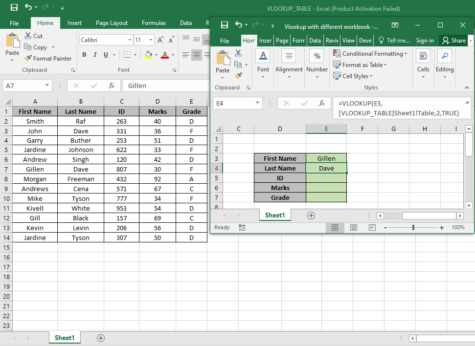
Here we have the table_array in Sheet1 of VLOOKUP_TABLE.xlsx.

Here we have a Table named range A2:E14. And we need to find the exact match Gillen with the first name in the Table.

Use the formula:

=VLOOKUP ( E3 , [VLOOKUP_TABLE] Sheet1! Table , 2 , TRUE )

E3 : Lookup_Value.

[VLOOKUP_TABLE] Sheet1! Table : Complete address of the vlookup table.

2 : look in the Second column of the Table.

TRUE : extracts only exact match.

As you can see the first match with Gillen. Now we can find all the corresponding values by the First Name basis

Replace the col_index_number from 2 to 3, 4 & 5 to get the rest of the values.

As you can see we got all the values, we needed which matches our exact lookup value.

Access Different Sheets in same workbook

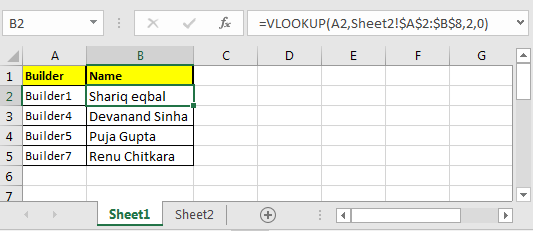
On sheet1 i have builder id. On sheet 2 i have name of those builders. So I just need to fetch name from sheet2 to sheet1 using VLOOKUP.

Write this formula in cell B2 on sheet1.

=VLOOKUP(A2,Sheet2!$A$2:$B$8,2,0)

Note the sheet2 here. If you rename it to sheet3, VLOOKUP will look for data on sheet 3 at range $A$2:$B$8 (locked the reference to range) if it exists other wise #REF error will be shown.

Here are some observational notes using the formula/method to access different workbook or sheets.

Notes:

The function returns error if workbook address is invalid or wrong.
The function returns the error if the value is not matched.

Hope this article about How to Link references with another workbook in Excel is explanatory. Find more articles on lookup formulas and related Excel formulas here. If you liked our blogs, share it with your friends on Facebook. And also you can follow us on Twitter and Facebook. We would love to hear from you, do let us know how we can improve, complement or innovate our work and make it better for you. Write to us at info@exceltip.com.

Related Articles:

Use INDEX and MATCH to Lookup Value : The INDEX-MATCH formula is used to lookup dynamically and precisely a value in a given table. This is an alternative to the VLOOKUP function and it overcomes the shortcomings of the VLOOKUP function.

Use VLOOKUP from Two or More Lookup Tables : To lookup from multiple tables we can take an IFERROR approach. To lookup from multiple tables, it takes the error as a switch for the next table. Another method can be an If approach.

How to do Case Sensitive Lookup in Excel : The excel's VLOOKUP function isn’t case sensitive and it will return the first matched value from the list. INDEX-MATCH is no exception but it can be modified to make it case sensitive. Let’s see how…

Lookup Frequently Appearing Text with Criteria in Excel : The lookup most frequently appears in text in a range we use the INDEX-MATCH with MODE function. Here's the method.

Popular Articles :

How to use the IF Function in Excel : The IF statement in Excel checks the condition and returns a specific value if the condition is TRUE or returns another specific value if FALSE.

How to use the VLOOKUP Function in Excel : This is one of the most used and popular functions of excel that is used to lookup value from different ranges and sheets.

How to Use SUMIF Function in Excel : This is another dashboard essential function. This helps you sum up values on specific conditions.

How to use the COUNTIF Function in Excel : Count values with conditions using this amazing function. You don't need to filter your data to count specific values. Countif function is essential to prepare your dashboard.