In my recent article, I talked all about named ranges in excel. While exploring named ranges, the topic of dynamic ranged popped up. So in this article, I will explain, how can you make Dynamic Range in Excel.

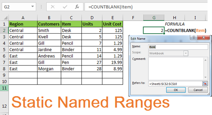
A normal named range is static. If you define C2:C10 as Item, Item will always refer to C2:C10, until and unless you edit it manually. In below image, we are counting blanks in the Item list. It is showing 2. If it were dynamic it would have shown 0.

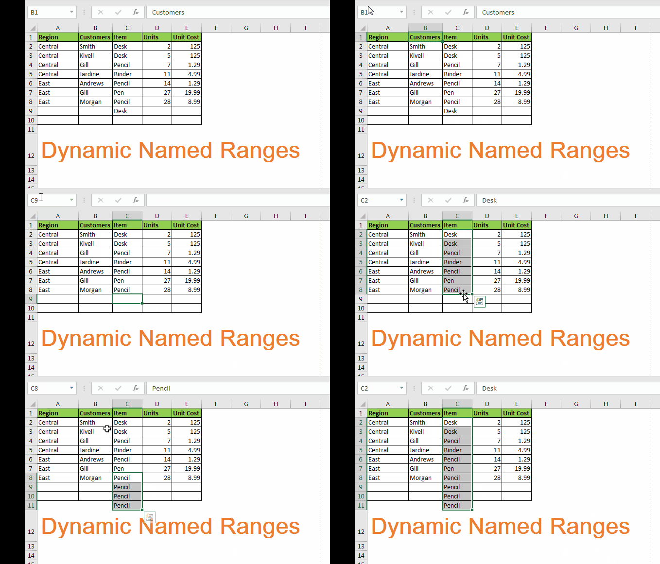
A dynamic name range is name range that expands and shrinks according to data. For example if you have a list of items in range C2:C10 and name it Items, it should expand itself to C2:C11 if you add a new item in range and should shrink if you reduce when you delete as above.
Create Named Ranges Using Excel Tables
Yes, excel tables can make dynamic named ranges. They will make each column in a table named range that is highly dynamic.
But there is one drawback of table names that you can’t use them in Data Validation and Conditional Formatting. But specific Named ranges can be used there.
To make a name range dynamic, we can use INDIRECT and COUNTA function
. How? Lets see.
Generic Formula to be written in Refers To: section
Above generic formula may look complex but it is easy actually. Let’s see by an example.
The basic idea is to determine last used cell.
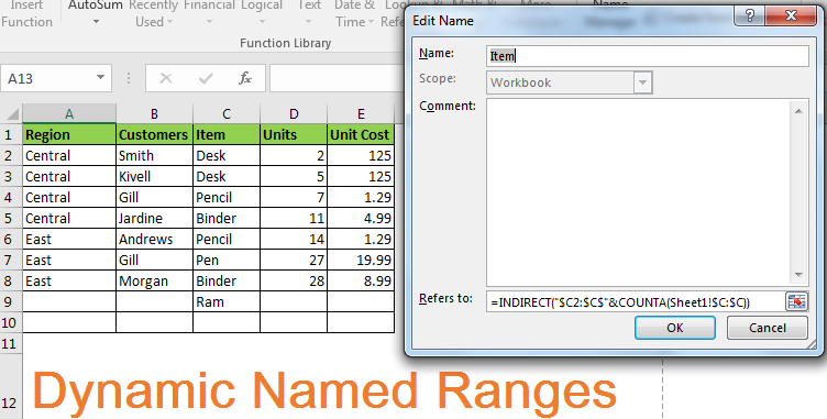
In above example we had an static name range Item in range C2:C10. Let’s make it dynamic.

And it's done. Now, whenever you will type Item in name box or in any formula it will refer to C2 to last used cell in the range.

Caution: No cell should be blank in-between range. Otherwise, the range will be reduced by the number of blank cells.
As I said, its only matter finding last used cell. For this example, no cells should be blank in between. Why? You’ll Know.
INDIRECT function in excel converts a text into range. =INDIRECT(“$C$2:$C$9”) will refer to absolute range $C$2:$C$10. We just need to find the last row number dynamically (9).
Since all cells have some value in range C2:C10, we can use COUNTA function to find the last row.
So,=INDIRECT("$C2:$C$"& this part fixes the starting row and column and COUNTA($C:$C) dynamical calculates last used row.
So yeah, this is how you can make the most effective Dynamic Named Ranges that will work with every formula and functionality of Excel. You don’t need to edit your named range again when you change data.
Download file:
Related Article:
How to use Named Ranges in Excel
17 Amazing Features of Excel Tables
Popular Articles:
50 Excel Shortcuts to Increase Your Productivity
How to use the VLOOKUP Function in Excel
The applications/code on this site are distributed as is and without warranties or liability. In no event shall the owner of the copyrights, or the authors of the applications/code be liable for any loss of profit, any problems or any damage resulting from the use or evaluation of the applications/code.