How to use the CHOOSE Function in Excel

In this article, we will learn about how to use the CHOOSE function in Excel.

SELECT from given list

Choose and return one value from a list of values. For example if we want to mark a quarter year with text values like 1st quarter, second quarter, Third quarter and fourth quarter on the database based on date value. Divide among 4 quarters and select from the list based on the given date value condition. Let's understand how CHOOSE function syntax works and some examples to illustrate the function usage.

CHOOSE Function in Excel

Excel CHOOSE function takes values and returns the value corresponding to a particular index_num.

CHOOSE Function Syntax :

=CHOOSE ( index_num , value1, [value2], ...)

Index_num : number corresponding to the required value

Value1 : first value

Value2 : second value

Example :

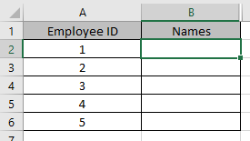
All of these might be confusing to understand. Let's understand how to use the function using an example. Here we have some employee ID and we need their names.

Use the formula in B2 cell to get the first name (value) form the list:

=CHOOSE(A2, "Anthony", "Andrew", "David", "Michelle")

A2 : index_num

Anthony : value 1

Andrew : value 2

Michelle : value 3

As you can see from the above snapshot that values are called using index_num in argument.

Copy the formula in other cells using the Ctrl + D shortcut key.

This is how CHOOSE function retrieves values from the values as arguments.

CHOOSE function usually used with other functions

We will use the combination with Mathematical functions like the SUM function. Here we have some values and needs to find the SUM of values in column B.

Use the formula:

=SUM ( CHOOSE ( 2 , A1:A10, B1:B10, C1:C10,))

Explanation:

The CHOOSE function will calls the second value

This will drop down to : =SUM(B1:B10)

We will use a Combination of CHOOSE with DATE & TIME functions like MONTH function.

Use the function

=CHOOSE(MONTH(A4),"Jan","Feb","Mar","Apr","May","Jun","Jul","Aug","Sept","Oct","Nov","Dec")

Explanation:

MONTH function returns a number and the number will be the index_num for the CHOOSE function.

Values corresponding to the number will be the return value of the formula.

As you can see here, you can rename the Month names as per your convenience.

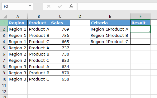
We will use a Combination of CHOOSE with LOOKUP functions like VLOOKUP function.

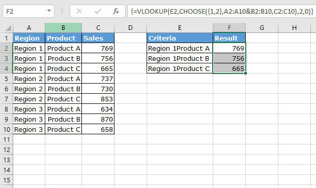
Use the formula in F2 cell:

{ =VLOOKUP (E2, CHOOSE ({1,2}, A2:A10 & B2:B10, C2:C10), 2, 0) }

Note : Do not try to put curly braces manually. Use Ctrl + Shift + Enter

As you can see CHOOSE function is very helpful when combined with other functions.

Here are all the observational notes using the CHOOSE function in Excel
Notes :

The function works with both numbers and text.
Change the format of the required result.
Index_num only be a number value from 1 to total count of value is listed.
Use the array reference with absolute char ($) for the array of values to be fixed,
Use carefully while using array of values.

Hope this article about How to use the CHOOSE function in Excel is explanatory. Find more articles on calculating values and related Excel formulas here. If you liked our blogs, share it with your friends on Facebook. And also you can follow us on Twitter and Facebook. We would love to hear from you, do let us know how we can improve, complement or innovate our work and make it better for you. Write to us at info@exceltip.com.

Related Articles :

How to Use TRIM function in Excel: The TRIM function is used to trim strings and clean any trailing or leading spaces from string. This helps us in the cleaning process of data a lot.

How to use the CLEAN function in Excel: Clean function is used to clean up unprintable characters from the string. This function is mostly used with the TRIM function to clean up imported foreign data.

Replace text from end of a string starting from variable position: To replace text from the end of the string, we use the REPLACE function. The REPLACE function uses the position of text in the string to replace.

How to Check if a cell contains one of many texts in Excel: To find check if a string contains any of multiple text, we use this formula. We use the SUM function to sum up all the matches and then perform a logic to check if the string contains any of the multiple strings.

Count Cells that contain specific text: A simple COUNTIF function will do the magic. To count the number of multiple cells that contain a given string we use the wildcard operator with the COUNTIF function.

Excel REPLACE vs SUBSTITUTE function: The REPLACE and SUBSTITUTE functions are the most misunderstood functions. To find and replace a given text we use the SUBSTITUTE function. Where REPLACE is used to replace a number of characters in string…

Popular Articles :

How to use the IF Function in Excel : The IF statement in Excel checks the condition and returns a specific value if the condition is TRUE or returns another specific value if FALSE.

How to use the VLOOKUP Function in Excel : This is one of the most used and popular functions of excel that is used to lookup value from different ranges and sheets.

How to use the SUMIF Function in Excel : This is another dashboard essential function. This helps you sum up values on specific conditions.

How to use the COUNTIF Function in Excel : Count values with conditions using this amazing function. You don't need to filter your data to count specific values. Countif function is essential to prepare your dashboard.