How to Get All Matches in Different Columns

031

This article will talk about how to get all values matched from a table and retrieve them in different cells. This is similar to lookup multiple values.

Generic Formula

{=INDEX(names,SMALL(IF(groups=group_name,ROW(names)-MIN(ROW(names))+1),COLUMNS(expanding ranges))), “--List Ends--”)}

Too many functions and variables!!!. Let's see what these variables are.
Names: This is the list of names.
Groups: The list of group to which these names belong too.
Group_name: the reference of group name.
Expanding ranges: this is the an expanding range that is used to get increasing number when copied to the right.

Example: Extract employees' names in different columns according to their company.
030
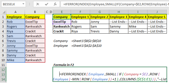
Let’s say you have a table of employees that is grouped according to their company. The first column contains employee names and the second column contains the name of the company.
Now we need to get each employee's name in different columns according to their company. In other words, we need to ungroup them.
Here, I have named A2:A10 as Employee and B2:B10 as Company, so that formula is easy to read.
Write this array formula in F2. Use CTRL+SHIFT+ENTER to enter this formula.

{=INDEX(Employee,SMALL(IF(Company=$E2,ROW(Employee)-MIN(ROW(Employee))+1),COLUMNS($E$1:E1))), “--List Ends--”)}

Copy this formula in all the cells. It will extract each individual name in the different columns according to their group.
031
As you can see in the image above, each employee is segregated in different cells.

So, how this formula works?
To understand the formula, let’s look at the formula in G2
Which is =IFERROR(INDEX(Employee,SMALL(IF(Company=$E3,ROW(Employee)-MIN(ROW(Employee))+1),COLUMNS($E$1:F2))),"--List Ends--")

The mechanics are simple and almost the same as multiple VLOOKUP formula. The trick is to get the index number of each employee from different groups and pass it to the INDEX formula. This is done by this part of the formula.

IF(Company=$E3,ROW(Employee)-MIN(ROW(Employee))+1):
This part returns an array of indexes and false for company name in $E3, which contains “Rankwatch”.
{FALSE;2;FALSE;4;FALSE;FALSE;7;FALSE;9}.
How? Let’s tear down it from inside.

Here we match the company name in $E3 with each value in Company range (Company=$E3).
This returns an array of true and false.{FALSE;TRUE;FALSE;TRUE;FALSE;FALSE;TRUE;FALSE;TRUE}.
Now the IF function runs it’s TRUE statements for TRUE, which is ROW(Employee)-MIN(ROW(Employee))+1. This part returns this part returns an array of indexes starting from 1 to number of employees {1;2;3;4;5;6;7;8;9}. The if function pics up values for only TRUE which in turn gives us {FALSE;2;FALSE;4;FALSE;FALSE;7;FALSE;9}.

The current formula is simplified to
=IFERROR(INDEX(Employee,SMALL( {FALSE;2;FALSE;4;FALSE;FALSE;7;FALSE;9},COLUMNS($E$1:F2))),"--List Ends--"). As we know small function return nth smallest value from an array. COLUMNS($E$1:F2) this returns 2. The SMALL function returns the second smallest value from the array above, which is 4.
Now the formula is simplified =IFERROR(INDEX(Employee,4),"--List Ends--"). Now, INDEX function simply returns the fourth name from employee array which gives us “Sam”.

So yeah, this how extract names from groups in different columns using INDEX, SMALL, ROW, COLUMNS and IF function. If you have any doubt regarding this function or if it is not working for you, let me know the comments section below.

Download file:

How to Get All Matches in Different Columns