We know how to do approximate match with VLOOKUP. But how do we do approximate match using INDEX MATCH? In this very article, we will learn, in excel how to do approximate match using INDEX and MATCH.
Generic Formula for Approximate Match
Result_array : The index from which you want to get result.
Lookup_value: the value which you are looking for in lookup_array.
Lookup_array: The array in which you will look for lookup value:
Note: The lookup table must sorted in ascending order to get correct answers.
Let’s learn by an example.
Example: Do an Approximate INDEX MATCH to get grades
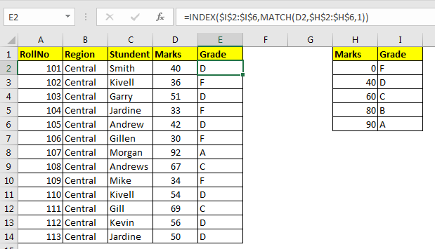
Here I have a list of students with their obtained marks in routine test. I need to give grades to these students according to another table. 0 to 39 as F, 40 to 59 D, 60 to 79 C, 80 to 89 B and 90 or above as A.
Note that the lookup table (marks and grade) is sorted ascendingly.

Write this formula in E2 and copy it down.

How it works?
Well this formula is using MATCH’s functionality of doing approximate match in the range. Actually, when we supply 1, TRUE or nothing to MATCH function, it performs an approximate match for lookup value. It means, if it doesn’t finds the given value in lookup range, it returns the last value found that was less than the given number.
So if we look at the formula in E3, it is
INDEX($I$2:$I$6,MATCH(D3,$H$2:$H$6,1))
The MATCH function looks for value of D3 (36) in range H2:H6. It fails to find 36 in range. So it returns the index of last value found in H2:H6 which is less than 36. And that value is 0 and its index is 1. Hence MATCH(D3,$H$2:$H$6,1) this translates to 1 in E3.
Now we have formula INDEX($I$2:$I$6,1). And this returns F.
So yeah guys, this how you do an approximate match using INDEX and MATCH function in excel. If you have any doubt about this or any other topic from excel 2019, 2016, and 2013 or older, let me know the comments section below.
Download file:
Related Articles:
Use INDEX and MATCH to Lookup Value
How to Use LOOKUP function in Excel
Lookup Value with Multiple Criteria
Popular Articles:
The applications/code on this site are distributed as is and without warranties or liability. In no event shall the owner of the copyrights, or the authors of the applications/code be liable for any loss of profit, any problems or any damage resulting from the use or evaluation of the applications/code.