How to Get Quarter of Year From Date

In this article, we will learn to generate random text values in  Excel.

For this article we will be needing the use of the following functions:

1. CHOOSE function
2. MONTH function

The following are the description & syntax for the functions used in the formula:

The CHOOSE function takes values and returns the value corresponding to a particular index_num.

The MONTH function takes a valid excel date as an argument and returns the month number (1-12) of the date. 

As we know, the MONTH function returns a number between the 1 to 12 numbers (months of the calender year). The CHOOSE function will take that number and return the value corresponding to the number.

Use the formula:

Explanation: 

1. The MONTH function returns a number from 1 - 12 (calender month of the year) of the valid input date.
2. The CHOOSE function returns a corresponding value from the value array based on the number returned by the MONTH function.
3. The value array is set according to the required output. A quarter of the year can start from Jan, Apr, July or Oct. 

Let's test this formula via running it on an example

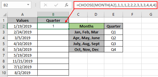
Here is our list of dates in Values column A2:A10.

Here we have given the quarter year sub section in the snapshot above. We need to find the quarter period of the date in Values using the formula shown below.

Use the formula:

Explanation:

1. The MONTH function returns a number from 1 - 12 (calender month of the year) of the valid input date.
2. The CHOOSE function returns a corresponding value from the value array {  1 , 1 , 1 , 2 , 2 , 2 , 3 , 3 , 3 , 4 , 4 , 4 } based on the number returned by the MONTH function.
3. Here The date is from January. The Month function returns 1. And the value corresponding to 1 is 1.

As you can see the function returns 1 means first quarter of the year.

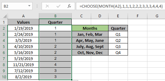
Here is the data that is provided as cell reference to the function. Now copy the formula to other cells using the Ctrl + D shortcut key or use the drag down option in Excel.

As you can see in the above snapshot the outcomes of the formula.

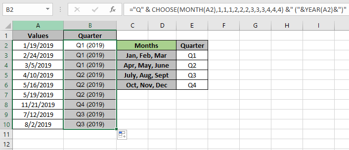
You can get the outcome with text like Q3 (year). Use the formula shown below.

Use the formula:

As you can see from the above snapshot the customized format for the outcomes.
Below are some of the observational outcomes of the formula.
Notes :

1. The CHOOSE function returns an error if the MONTH function returns anything else except the number from 1 - 12.
2. The MONTH function returns the error if the argument date provided is invalid date as per Excel.
3. The CHOOSE function returns #VALUE! Error if the value array argument to the function is given as array.

Hope this article about how to generate random text values in Excel is explanatory. Find more articles on TEXT functions here. Please share your query below in the comment box. We will assist you.

Related Articles

How to use the CHOOSE Function in Excel

How to use the MONTH Function in Excel

Find the nth root of a number

Calculate Weighted Average

Ignore zero in the Average of numbers

Popular Articles

50 Excel Shortcut to Increase Your Productivity

Edit a dropdown list

Absolute reference in Excel

If with conditional formatting

If with wildcards

Vlookup by date

Convert Inches To Feet and Inches in Excel 2016

Join first and last name in excel

Count cells which match either A or B