How to use the DVAR Function in Excel

In this article, we will learn about how to use the DVAR function in Excel. 

DVAR function is built-in database function in Excel. The DVAR function returns the Variance of the values from the sample database having multiple conditions. Conditions to the function is given using a table, which must have the same fields or headers as on the database.

DVAR function returns the Variance of the field based on given multiple criteria. The DVAR function takes criteria as a table having the same fields as on the database. 

Syntax:

database : database

field : the required field, call by name or text in quotes.

Criteria : one or more conditions taken as table array.

EXAMPLE:

This all might be confusing to you so lets gear up and understand the DVAR function using it in an example.

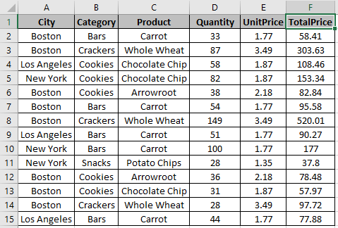
Database

Table

Here we have a list of Products bought with their respective details  & We need to get the Variance from the TotalPrice based on criterias mentioned in the table

There are some things you have to take care of when using this function

1. Database and criteria table should have same fields.
2. Formula must be used in any other cell than criteria area.

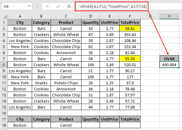
First condition is City : Boston

Second condition is Product : Carrot

So the function must return the Variance of the Carrot (Product) bought from Boston (city)

Use the formula for the above condition:

A1 : F15 : database 

"TotalPrice" : field by text in quotes or field can be input as 4 (4th column from the database).

A17 : F18 : criteria as table array

The Variance of the values comes out to be 690.804 .

DVAR function can have multiple criteria on one field by adding rows in the table

Now we will take an example taking multiple criteria on the same database.

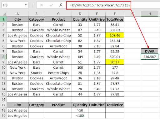
Here we have multiple conditions on the field Quantity i.e. less than 100 & greater than 50 units bought from Los Angeles. We need to get the Variance of TotalPrice having the conditions stated in the snapshot.

Use the formula for the above condition:

A1 : F15 : database 

"TotalPrice" : field by text in quotes or field can be input as 6 (6th column from the database).

A17 : F19 : multiple criteria by adding one row in table array

The Variance of the values comes out to be 236.587 .

You don’t need to edit the formula every time as criteria field gets updated as soon as  you provide the input to table fields.

Notes:

1. Wildcards keys ( * , ? , ~ ) can be used with the DVAR function.
2. The function returns an error if any field value is incorrect.
3. If data represents a sample, use the DVAR function. DVARP function is used to calculate the Variance for an entire population. 

As you can see the DVAR function in excel returns values from the table field.

Hope you understood How to use the DVAR function in Excel. Explore more articles on Mathematical functions like VAR and VARP functions here. Please state your query or feedback in the comment box below.

Related Articles

How to use the DCOUNT function in Excel

How to use the DSUM function in Excel

How to use the DAVERAGE Function in Excel

How to use the DMAX Function in Excel

How to use the DMIN Function in Excel

How to use the DPRODUCT Function in Excel

How to use Wildcards in Excel

Popular Articles

50 Excel Shortcut to Increase Your Productivity

Edit a dropdown list

Absolute reference in Excel

If with conditional formatting

If with wildcards

Vlookup by date

Join first and last name in excel

Count cells which match either A or B