How to Get Maximum Value From a List Having Errors

In this article, we will learn about how to get the Maximum score from the list having error values in Excel 2013.

Scenario:

For instance, we have a list of numbers having some errors in a list. We need to find the MAX number from the list. How can we obtain such values? Excel MAX function generates #NA error, if used. The below mentioned formula does exactly the same and get's the maximum value from a list, ignoring all errors.

Generic formula:

function - number, type of function to perform on array.
option - number, type of criteria to apply on array.
Array - list of scores or numbers.

The above two tables are guide to function and option selection.

Example:
Let’s see how can we get max values while ignoring errors, using it as an example.
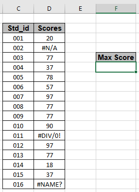
Here we have a Data Std_ID range from C3:C18 & a list of their respective scores in range D3:D18 as shown in the snapshot below.

We need to use the formula for the above stated problem.
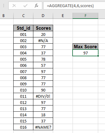
Use the formula:

Explanation:

1. AGGREGATE function performs many operations via selecting required operation number. 4 is the operation number for MAX function.
2. AGGREGATE function performs many criteria options via selecting the desired option. 6 is criteria or option_num for ignoring error values.
3. Scores is named range array used for the D3:D18 range.

The maximum of scores in list is 97. As you can see the formula returns max score from the list having error values.

As you must be working on Excel 2013 till. But if you working in EXCEL 2016 version then you have another option of using the MAXIFS function.
MAXIFS function returns the MAX value having criteria
Use the formula for EXCEL 2016:

As you can see you can get the MAX value from the list using the two functions explained above .

Here are some observational notes as mentioned below.

Notes:

1. Use the function_num argument carefully.
2. Use the Option_num argument carefully.
3. Use the named range of cell reference to give array as argument.

Hope you understood how to get the Maximum value from the list having errors in Excel. Explore more articles on Excel Count functions here. Please feel free to state your query or feedback for the above article.

Related Articles

How to use MAX function in excel: Use the MAX function to get the Maximum value from the array in Excel.

Calculate max if condition match : Get the MAX value from the array having criteria.

How to Use Excel AGGREGATE Function : Use the AGGREGATE function to perform multiple operation with multiple criterias in excel.

COUNTIFS With OR For Multiple Criteria : Count cells having multiple criteria match using the OR function.

How to use wildcards in excel : Count cells matching phrases using the wildcards in excel

Popular Articles

50 Excel Shortcut to Increase Your Productivity

Edit a dropdown list

If with conditional formatting

If with wildcards

Vlookup by date