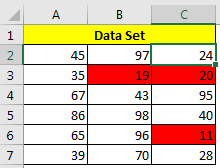
In data analysis and MIS reporting, we often get the need to highlight the top and bottom values. This helps us to easily identify focus areas. In this article, we will learn how we can highlight the 3 lowest values in Excel data set, using conditional formatting.
Let’s see an example to see how we can do this.
Example: Highlight 3 lowest values in a data set
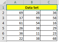
In range A2:C7 I have a formula =RANDBETWEEN(10,100). This formula generates a random number between 10 and 100, in each cell, whenever a change made in the file. I want to highlight the smallest 3 numbers in this range.

To highlight the smallest three value in excel, follow these steps:


This was easy. But things get a little bit tricky when we add another criteria for highlighting bottom values. Here I have prepared a tutorial on how to highlight lowest 3 values in range with criteria. Go check it out.
So, yeah this how you can highlight bottom 3 values in a range. Using this method you highlight n number of bottom values. There's no restriction in excel for that. If you have any doubts on this article or any other excel topic, mention it in the comments section below.
Related Articles:
Highlight Top 3 Values in a Range.
Highlight Bottom 3 Values in a Range with Criteria.
Conditional formatting based on another cell value
Conditional Formatting with formula 2016
Conditional Formatting using VBA in Microsoft Excel
Highlight cells that contain specific text
Popular Articles:
The applications/code on this site are distributed as is and without warranties or liability. In no event shall the owner of the copyrights, or the authors of the applications/code be liable for any loss of profit, any problems or any damage resulting from the use or evaluation of the applications/code.