A risk matrix is used to determine the risk in numbers using the impact and possibility index. Impact, possibility or certainty index can be any ascending or descending number.
So first we will need to create a risk matrix chart so that we can use it later in our analysis.
Let's start this article with the Risk Matrix Example directly without any generic formula.
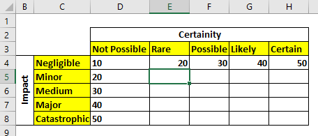
To use the risk matrix we need to create one first. You will need to prepare a table like the one below:

In rows, I have assigned the impact and in columns I have written the certainty. The first values assigned to certainty and Impact are arbitrary but in proper ascending order.
Now the rest of the matrix is filled by this formula= Certainty x Impact
So to fill the risk matrix, we will write this formula in cell E5 and copy it to other cells of the matrix.
| =$D5*E$4 |
I am using absolute referencing here.
Our risk matrix is ready.

Now that our RISK matrix is ready, let's learn how to retrieve values from it by providing Certainty and Impact text.
We can use the INDEX and MATCH function to retrieve values from this table.
The generic formula for retrieving the risk value will be:
| =INDEX(matrix,MATCH(certainty,certainty_headers,0),MATCH(impact,impact_headers,0)) |
Matrix: This is the entire matrix value range (excluding headers).
Certainty: This is the certainty level label.
Certainty_headers: This is the range that contains the certainty level labels.
Impact: This is an impact level label.
Impact_headers: This is the range that contains the impact labels.

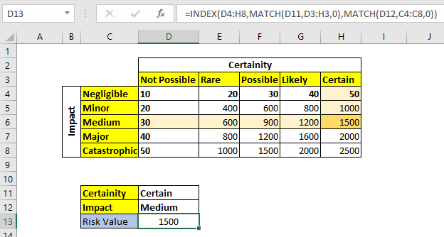
In the image above we have certainty levels in D11 and Impact level written in D12. We need to get the Risk value of this combination from the risk matrix above.
For this, we use the above mentioned generic formula in cell D13.
| =INDEX(D4:H8,MATCH(D11,D3:H3,0),MATCH(D12,C4:C8,0)) |
It returns 1500.

As you can see it has returned a risk value. This value can be used to make important decisions. Here we used a small matrix to illustrate the use. But in reality you may have a bigger matrix which can be used manually. In those cases, this formula will be a life saver.
How does it work?
The technique is quite simple. The INDEX function is used to retrieve value from a 2D array using the row and column index. We use the MATCH function to retrieve the row and column index for INDEX function. Here's how it is solved step by step:
| =INDEX(D4:H8,MATCH(D11,D3:H3,0),MATCH(D12,C4:C8,0)) |
| =>INDEX(D4:H8,5,3) |
| =>1500 |
In the first step both MATCH functions are solved. The first MATCH looks for "certain" (value in D11) in range D3:H3. It finds at 5th location and returns 5. Similarly, the second MATCH looks for the text "Medium" in range C4:C8. It finds it at 3rd position and returns. Finally, the INDEX function looks in the 5th column and 3rd row of array D4:H8 and returns 1500.
So yeah guys, this was a quick example of the Risk Matrix calculation in Excel. I hope it was explanatory enough and served your purpose of being here. If you have any questions regarding this article or anything else about Excel/VBA, let us know in the comments section below.
Related Articles:
Lookup nth match using INDEX & MATCH function | To get nth match without using a helper column we use INDEX and MATCH function. We use the boolean logic to get the index from the table.
How to LOOKUP Multiple Values | To retrieve all the matching values from a list, we use the INDEX MATCH function. VLOOKUP can retrieve multiple values only when we use a helper column.Lookup Value with Multiple Criteria | If you have to lookup more than one lookup tables then how do you use VLOOKUP from two Lookup tables or more. This article solves this problem very easily
Lookup Value with Multiple Criteria | We can simply use the VLOOKUP function. But when you don’t have that unique column in your data and need to lookup in multiple columns to match a value, VLOOKUP doesn’t help
How To Look Up Address in Excel | There will be times when you would want to get the address of the cell from which a value is being retrieved. Using that address you can easily retrieve adjacent values using the OFFSET function
Popular Articles:
50 Excel Shortcuts to Increase Your Productivity | Get faster at your task. These 50 shortcuts will make you work even faster on Excel.
How to use Excel VLOOKUP Function| This is one of the most used and popular functions of excel that is used to lookup value from different ranges and sheets.
How to use the Excel COUNTIF Function| Count values with conditions using this amazing function. You don't need to filter your data to count specific values. Countif function is essential to prepare your dashboard.
How to Use SUMIF Function in Excel | This is another dashboard essential function. This helps you sum up values on specific conditions.
The applications/code on this site are distributed as is and without warranties or liability. In no event shall the owner of the copyrights, or the authors of the applications/code be liable for any loss of profit, any problems or any damage resulting from the use or evaluation of the applications/code.