How to extract unique values through Excel formula?
To count the unique values from a list, we use the IF function along with the COUNTIF function in Microsoft Excel 2010.
IF: -The IF condition allows you to check for multiple conditions in a cell. It helps us to create the flexibility of the function in Microsoft Excel 2010 & 2013. Excel allows us to use upto 64 conditions which can be checked in a cell.
Syntax of IF function: =IF(logic_test, value_if_true, value_if_false)
COUNTIF: The COUNTIF function is used to count the number of cells in a range, which meet a given criteria.
Syntax of COUNTIF function: =COUNTIF(range, criteria)
Let’s consider an example to understand how to retrieve the unique list or unique count in Excel:-
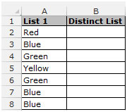
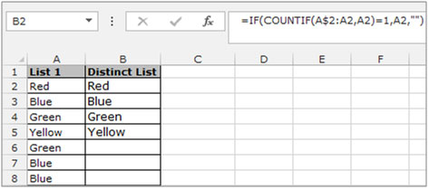
Example 1: I have a list of color names in range A2:A8, in column B I want to extract a distinct list of color names.

Follow the below given steps:-

The applications/code on this site are distributed as is and without warranties or liability. In no event shall the owner of the copyrights, or the authors of the applications/code be liable for any loss of profit, any problems or any damage resulting from the use or evaluation of the applications/code.
Is there a way to make a formula to help identify, and possibly delete, duplicates under 3, while keeping the log names that show up more than 3? There will be duplicates of almost every log name, but I need to remove any that don't have a duplicate of 3 or more. The log names are all within a single column, such as "A" or "B" only. I have two separate log name columns that can be used, one column is number based, the other column is word based. Both the number and word column are attached to each other in each row if that helps.
You can use as well a matricial formula to get a good results.
Imagine you have a list starting in cell B2 with 20 names.
{=IFERROR(INDEX($B$2:$B$21;MATCH(0;COUNTIF($C$1:C1;$B$2:$B$21);0));"")}
COUNTIF - will return all different numbers from the above cell.
MATCH - is considering when it find a new number that is represented by "0" in the first parameter, this new number is returned as result.
INDEX - it is the matrix that we want to remove the duplicated datas.
IFERROR - To remove errors message when it runs all over the list.
Don't forget to push "ctrl+shift+enter" to apply the matricial formula.
José Córdoba Cáceres Junior, first of all, this is one of most smart, simple and usefull formulas I've ever seen. Congrats! A question... How do I add a new criteria in the formula. I.e., let's imagine that I have a column D, named as Status. I'd like to list the names, as you did, but with Status = "Normal".
Dear Sir,
this formula =IF(COUNTIF(A$2:A2,A2)=1,A2,””)
is vary help full
but it is showing empty cells in middle, how to sort the data automatically
regards
kamaraj
How if there are blank cells in between the values in a column?
Thanks for the article, it's extremely helpful. How could I modify the formula to allow for a second criteria? I have tried several variations but can't get it to work. Logic would be something like where it shows all unique values of Column B where column A=X.
A1=A3*50*1.15
A2=0.0665*2*(100-60)/6.5*(60-40)
A3 shall be choosen from column A4, which is array of 5, 10, 15, 20, and so on.
The value choosen shall give the result that A1 should be greater than A2. if anyone have formula in their knowledge please share with me.
Regards
Vishu
E4: =ROWS($B$4:B4)
F4: =IF(B4=A4;E4;"")
G4: =IFERROR(SMALL($F$4:$F$11;E4);"")
K4: =IFERROR(INDEX($A$4:$B$11;$G4;COLUMNS($K$3:K3));"")
Pull formulas down.
This formula, while it does de-duplicate, does not provide a nicely ordered list. You'd need another column to do that.
How to I do that?