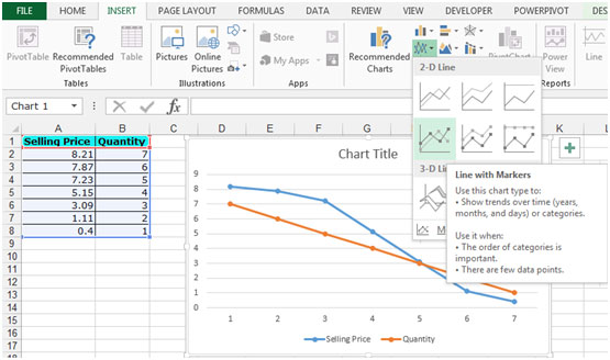
How to Change the Value of X Axis in Microsoft Excel 2010

If we need to change the value of the X-Axis or any axis of the chart, , we have to first prepare a chart in Microsoft Excel 2010. This will help us understand the steps involved.
.
Let’s take an example and understand: - We have data in range A1: B8, in which column A contains selling price and column B contains quantity. We will create a line chart.

To create the line chart in excel follow the below mentioned steps:-

Select the data A1:B8.
Go to the “Insert” tab, and select the Line with Marker chart from the “Charts” group.

Right clickonthe mouse and select Chart>Select Data.

On the left side in the “Legend Entries (Series)” box uncheck “Quantity” and click on ok. The chart will show the data only for the Selling Price.

To change the value of X Axis follow the below mentioned steps:-

Click on the Chart.
Right click on the mouse and select chart > Select Data.
The “Select Data Source” dialog box will appear.
On the left side in the “Legend Entries (Series)” box check on “Quantity” and uncheck on“Selling price”.