Formula to change Font Color in Microsoft Excel 2010

If we want to change the font color of some cells to show some noticeable difference between the cells, we can do this using conditional formatting.

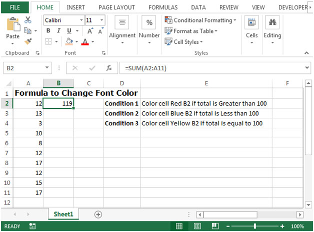
• We have few random numbers in cells A2:A11
• The sum of these cells is calculated in cell B2.
• We have defined three conditions in column E in the below picture.
• If the value in cell B2 meets the condition then the font color will change automatically.

See the below picture

Lets see how we can use conditional formatting to show a value with different font colors according to the defined conditions:

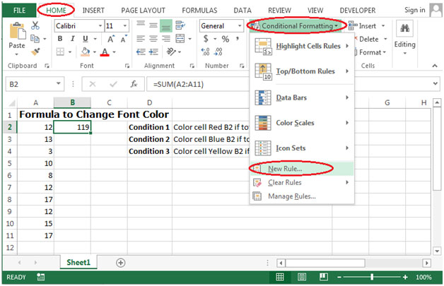
• Select cell B2 where the font color needs to be changed. Click on the Home tab on the Ribbon, select Conditional Formatting & then New Rule

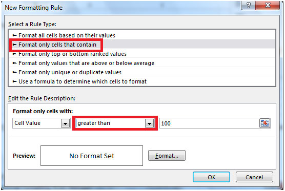
• On selecting New Rule, the New Formatting Rule dialog box will appear. Then select Format only cells that contain

• Select Cell Value greater than 100 which is our condition
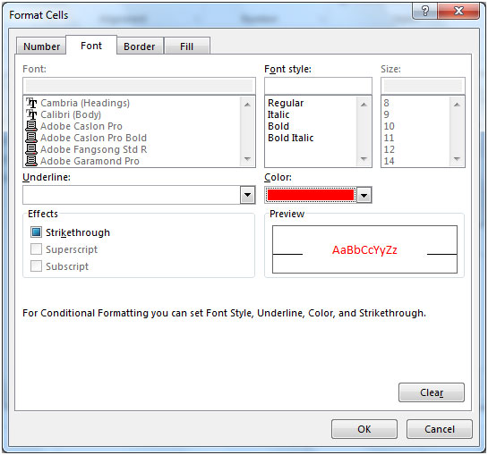
• Click on the Format button, then click on the Font tab and choose the color from the drop down. Letsselect Red.

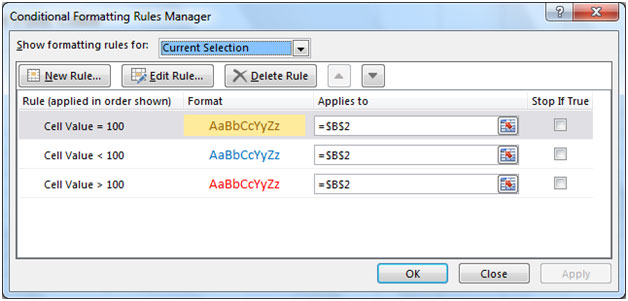
• Follow the above steps again for other conditions for the Blue & Yellow colors. Ensure that you change the parameter from greater than to less than 100 for blue and equal to 100 for yellow.

• Click on Ok
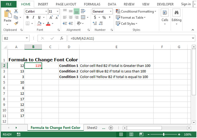
• We will get our output as the below picture.