Minimum value based on the criteria in microsoft excel

In this article, we will learn about how to find the minimum value if it matches multiple conditions in Excel.

Scenario:

When working with long ranges of data, we need to find the minimum value among the range where more than one condition is matching. In simple words finding out the minimum value using Excel IF function. IF function returns True or False and MIN function looks for the minimum value from the corresponding array.

Syntax to find min with multiple criteria

{=MIN (IF (Criteria1=match1),IF(Criteria2=match2, range_min))}

Note: Use Ctrl + Shift + Enter when working with arrays or ranges in Excel. This will generate Curly Braces on the formula by default. DO NOT try to hard code curly braces characters.

Example:

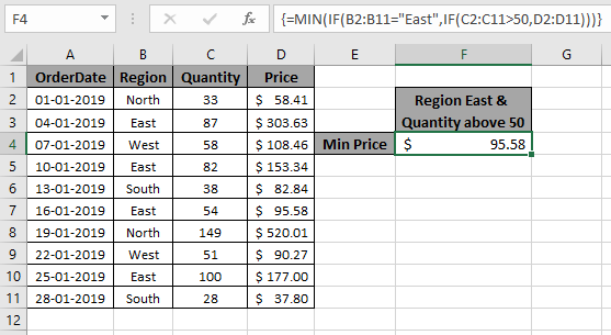
All of these might be confusing to understand. So, let's test this formula via running it on the example shown below. Here we will perform the formula over values with given criteria.

Use the formula:

{ =MIN( IF( B2:B11="East", IF( C2:C11 > 50 , D2:D11 )))}

criteria 1 is price must be from the region "East"

criteria 2 is price where quantity is greater than 50.

Explanation:

IF( C2:C11 > 50 , D2:D11 ) returns an array of FALSE values and price values where quantity is greater than 50.

{ FALSE ; 303.63 ; 108.46 ; 153.34 ; FALSE ; 95.58 ; 520.01 ; 90.27 ; 177 ; FALSE }

IF( B2:B11="East", IF( C2:C11 > 50 , D2:D11 )) returns an array of remaining price values where region is East.
MIN function finds the minimum value from the returned array and that would be the required PRICE value.

Here we matched the range (B2:B11) with value "East" and quantity (C2:C11) greater than 50, which returns the minimum from the price range (D2:D11). Press Enter to get the minimum of the range

As you can see we have the MIN value, if criteria match from the range of values.

Alternate function for Excel 365 and 2019 version.

The Excel MINIFS function is a new function, introduced in Excel 365 and 2019. This function returns the minimum value from a given range.

In this article, we will learn how to use the MINIFS function in Excel.

Syntax of MINIFS Function

=MINIFS(min_range,criteria_range1,criteria1,...)

Min_range1: It is the numeric range that contains the minimum value.

Criteria_range1: It is the criteria range that you want to filter before getting the minimum value.

Criteria1: It is the criteria or the filter that you want to put on criteria_range before getting the minimum value.

You can have multiple pairs of criteria_range and criteria.

Let’s understand the MINIFS function with an example.

Example of MINIFS Function

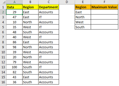
So, here I have a table of some data. The first column contains the numeric values. Second column contains the Region and the third column has the department.

The task is to tell the min value from the first range for each region.

The formula for getting maximum value from "East" region will be:

=MINIFS(A2:A16,B2:B16,"East")

It will return 29.

Here we have given hardcoded criteria, but we can also give reference of the criteria to make it dynamic.

=MINIFS($A$2:$A$16,$B$2:$B$16,E2)

Here we have used absolute ranges to lock the min_range and criteria_range.

You can put more than 1 criteria in MINIFS function. For example, if I want to get minumum value from IT department of SOUTH region then the formula will be:

=MINIFS(A2:A16,C2:C16,"IT",B2:B16,"SOUTH")

This will return 36 as per above data. If we put "Accounts" in place of IT, the MINIFS will return 82.

Here are some observational notes using the above formula.

Notes:

The formula returns the min value from the range.
Use MINIFS function in MS Excel 365 version to get the minimum value from data having multiple criteria. Learn more about MINIFS function here.
Named range in the formula be used with correct keywords.

Hope this article about Minimum value based on the criteria in microsoft excel is explanatory. Find more articles on IF condition formulas here. If you liked our blogs, share it with your fristarts on Facebook. And also you can follow us on Twitter and Facebook. We would love to hear from you, do let us know how we can improve, complement or innovate our work and make it better for you. Write to us at info@exceltip.com.

Related Article

Calculate minimum if condition match in Excel 2016 | To calculate the minimum value with a condition in Excel 2016 and older versions, use this formula. Using the MIN and IF function together we can get a conditional minimum output.

Excel 2019/365 Functions:

How to Use The Excel UNIQUE Function | The UNIQUE function returns the Unique values from the given array.

The SORT Function in Excel | The SORT function returns the sorted form of the supplied array.

How to Use Excel SORTBY Function | The SORTBY function sorts a given range by a different specified range. Sorting range does not need to be part of the table.

How to Use The Excel FILTER Function | The FILTER function returns all matched values of given criteria and spills the result into adjacent cells.

The SEQUENCE Function in Excel | The SEQUENCE function returns a series of sequential numbers. It is a dynamic array formula.

Popular Articles :

How to use the IF Function in Excel : The IF statement in Excel checks the condition and returns a specific value if the condition is TRUE or returns another specific value if FALSE.

How to use the VLOOKUP Function in Excel : This is one of the most used and popular functions of excel that is used to lookup value from different ranges and sheets.

How to Use SUMIF Function in Excel : This is another dashboard essential function. This helps you sum up values on specific conditions.

How to use the COUNTIF Function in Excel : Count values with conditions using this amazing function. You don't need to filter your data to count specific values. Countif function is essential to prepare your dashboard.