Pivot Table Report - Grouping the Date Field by Days, Months, Quarters and Years in Microsoft Excel 2010

To create a pivot table report – grouping the date field by days, months, quarters and years, let us first create a pivot table report.

Let us take an example:

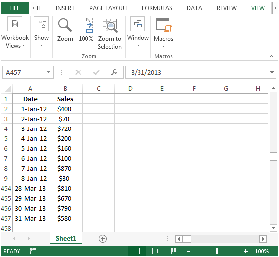
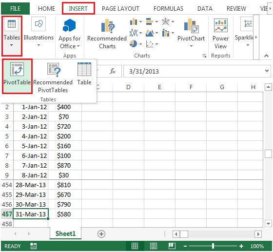
• We have dates in column A from 1-Jan-2012 to 31-Mar-2013

• Click on Insert Ribbon to create a pivot table report
• In Tables group, click on Pivot Table.

• The following dialog box will appear

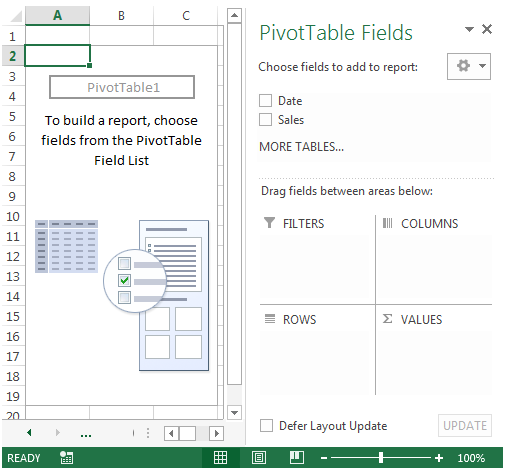
• Select existing worksheet option if you want to create the report in existing worksheet, otherwise click on OK to create in new worksheet.

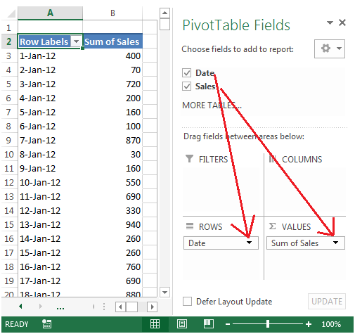
• Drag Date to Rows field & Sales to Values field.

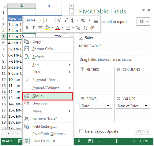
• Now you need to click on any cell in column A (Date column) & right click and select Group option

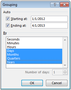
• Select Days, Months,

  Quarters & Years as show below in snapshot

• Click on OK, and you will see the Sales will segregated per date wise.

Grouping the dates will allow you to quickly find the sales in a particular period.