Perform Conditional formatting based on another cell value in excel

In this article, we will learn about how to use Conditional formatting based on another cell value in Excel.

In simple words, We need to view highlighted data on the basis of values in another cell. Conditional Formatting is used to highlight the data on the basis of some criteria. It would be difficult to see various trends just for examining your Excel worksheet. Conditional Formatting provides a way to visualize data and make worksheets easier to understand. It also allows you to apply formatting basis on the cell values such as colours, icons and data bars. For this, we will create a rule in Conditional Formatting.

Example:

Let’s understand this function using conditional formatting in an example.

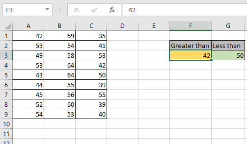
Here we have some values on the left side on which conditional formatting is being applied.
And on the right side we have some values on which the conditional formatting values are based upon.
We need to follow some steps

Select the cells A1 : C9.

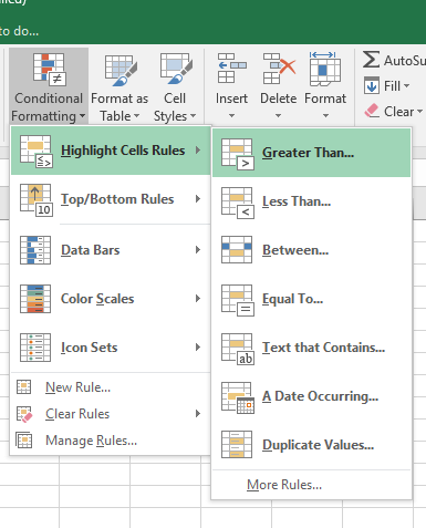
Go to Home > Conditional Formatting > Highlight Cells Rules > Greater Than..
A dialog box will appear in front

Select the F3 cell in the first bow and then select the formatting of the cells to Yellow Fill with Dark Yellow Text.

Click Ok.

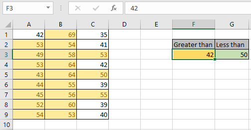
As you can see the format of values is changed using Conditional formatting.

You might also notice that what happened to the values between 42 & 50. Excel overwrites the first rule and give preference to the last rule applied. If you wish to highlight
the data with different colour. Make new rule in conditional formatting

Now we need to view the results based on another cell value.

For that go through the same process
Select the cells

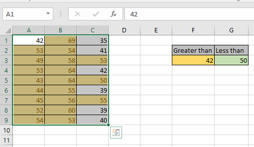
Go to Home > Conditional Formatting > Highlight Cells Rules > Less Than..

A dialog box will appear in front

Select the G3 cell in the first bow and select the formatting of the cells to Green Fill with Dark Green Text as shown in the snapshot below.

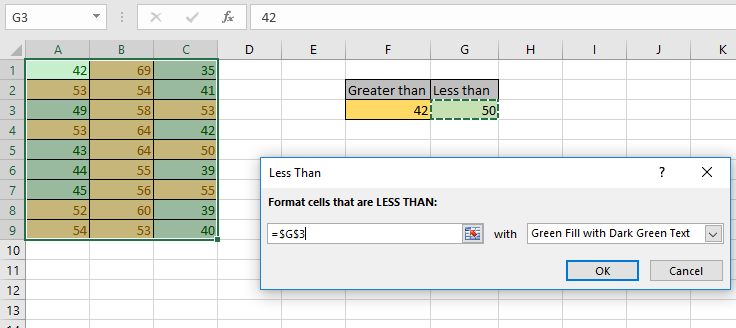
Click Ok.

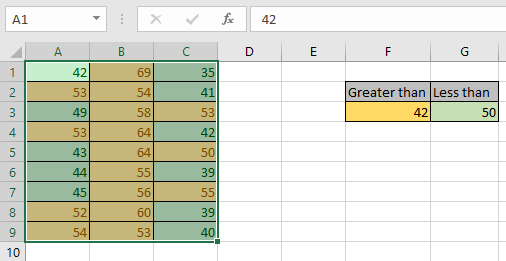
As you can see the new format of values is changed using Conditional formatting based on cell values.

Changing the values in the cell changes resulting cells.

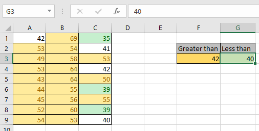
As you can see we changed the value in G3 cell from 50 to
40 and can view the updated results.

Hope you understood how to use Conditional formatting based on another cell value in Excel. Explore more articles on Excel Conditional formatting here. Please feel free to state your query or feedback for the above article.

Related Articles:

IF and Conditional formatting in Excel

Perform Conditional Formatting with formula in Excel

Perform Conditional Formatting using VBA in Microsoft Excel

Popular Articles:

50 Excel Shortcuts to Increase Your Productivity | Get faster at your task. These 50 shortcuts will make you work ODD faster on Excel.

The VLOOKUP Function in Excel | This is one of the most used and popular functions of excel that is used to lookup value from different ranges and sheets. 

COUNTIF in Excel 2016 | Count values with conditions using this amazing function. You don't need to filter your data to count specific values. Countif function is essential to prepare your dashboard.

How to Use SUMIF Function in Excel | This is another dashboard essential function. This helps you sum up values on specific conditions.