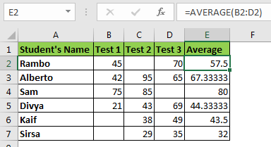
In this article, I will explain how you can format a cell if cell/s are blank in other columns. To understand this conditional formatting in excel let's have an example.
Example: Highlight Average Cell if Test Column is Blank

Here, I have data on test scores. I conducted three tests. In column E, I am calculating the average scores of students. In some cases, students have missed the test and I want to highlight the average score if the student has missed any test.
In Excel words, highlight the cell in column E if the adjacent cell of column B, C, or D is blank.

And it is done. You can see that the average scores are highlighted of those students who have missed any test.

How does it work?
Here we have used the COUNTBLANK function that counts the number of blank cells in a range.
In conditional formatting, any number greater than 0 is considered True.
Here the formula is COUNTBLANK($B2:$D2). We have locked columns and left rows relative. It makes column absolute and allows rows to change. Now, since B2:D2 contains a blank cell, the function returns 1. Which translates to TRUE. Hence we get a yellow filled average cell. In B3:D3, there's no blank cells and the function returns FALSE and the cell doesn't turn yellow.
ISBLANK Method
The same thing can be done with another formula.
The ISBLANK function returns TRUE if a cell is blank else it returns FALLS. If we add TRUE-FALSE values it acts like an OR function. So, if any function cell is blank the formula above will return TRUE. In return, the cell will be filled with yellow colour.
The same thing can be done with the formula below.
Another equivalent formula is
In the above two methods, we are checking individual cells if they are blank or not. We have encapsulated these checks with the OR function. As per the OR function property, it returns true if any of the tests return true.
So yeah, this is how you can do conditional formatting of the cells if a cell in other columns is blank. I hope this article was explanatory enough to explain the procedure of column conditional formatting in excel. You can click on the function names in the formula to read about that function. If you have any specific problem in excel, mention it in the comments section below.
Related Articles:
Conditional formatting based on another cell value
Conditional Formatting with formula 2016
Highlight cells that contain specific text
Popular Articles:
The applications/code on this site are distributed as is and without warranties or liability. In no event shall the owner of the copyrights, or the authors of the applications/code be liable for any loss of profit, any problems or any damage resulting from the use or evaluation of the applications/code.