How To Highlight Row in Excel if Row Contains Specific Text

Sometimes, we want to highlight the row that contains the specific text. In this article, we will learn how to highlight a row, if any cell in that row contains a specific text or value. We will highlight row using conditional formatting of course.

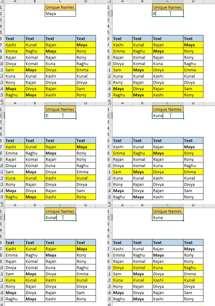
Generic Formula in Conditional Formatting

Lookup value: it is the criteria text. It will be searched in the given range.
Lookup array: the row that you want to highlight.
The first row need to be selected while applying the conditional formatting.
Let’s see an example to make things clear.
Example: Highlight Rows That Contain a Specific Text

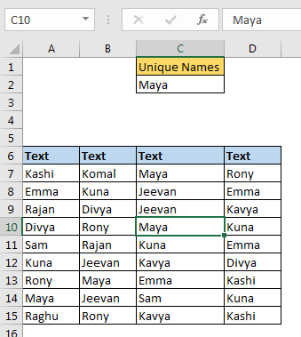
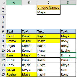
Here I have some data in table. Each row contains some random name. I want to highlight each row in table that contains the value written in C2. For now, in C2, I have Maya. I want to highlight each row that contains Maya in it.

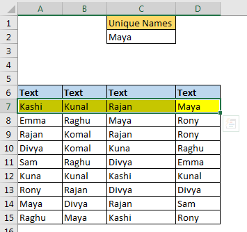
Select first row of the table (A7:D7).

1. Go to conditional formatting and click on the new rule. You can use sequential shortcut ALT>H>L>N.
2. Select “use a formula to determine which cell to format”.
3. Write this formula.
=MATCH($C$2,$A7:$D7,0)
4. Click on format and choose yellow infill. Hit ok.


Now the selected row is highlighted.

Copy this range and paste special the format to the entire table.

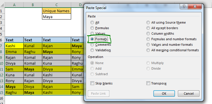
Now each row will be highlighted that contains “Maya”. When you change the value in C2, row containing that value will be highlighted only.

How it works?

Here, we used the MATCH function of excel that returns the index of the searched value in the given range. If it fails to find the given text, it returns #NA.

In conditional formatting, any positive value is treated as TRUE and Errors are treated as FALSE. We use this functionality to highlight row.

Here our formula is =MATCH($C$2,$A7:$D7,0). Note that the lookup value’s reference is absolute. So that it always looks for value written in C2. The lookup range is A7:D7. Note that only Columns are frozen using $ and rows are left relative. It is because we want to change the lookup row when we copy the conditional formatting and while columns are absolute. In the end, we get highlighted rows that contain specific text in a cell. Learn about referencing in detail here.

If we make column relative (=MATCH($C$2,A7:D7,0)) our rows will be highlighted to first found value.

The above formula highlights the rows that contain specific text. It checks cells and matches cells value. But if you want to check the given text in between of strings then you should use this function.

=SEARCH($C$2,$A7&$B7&$C7&$D7)

Here we are just searching for text in concatenated text of A7:D7. If SEARCH finds the given text, conditional formatting treats it as TRUE else False. Rest is same as above.

Highlight Row with Case Sensitive Match

For case sensitive match, we can use FIND function. This will check text and in rows and it will highlight the row only if text and case is matched.

=FIND($C$2,$A7&$B7&$C7&$D7)

So yeah guys, this is the way you can highlight a row base on a  text match. Let me know if you have any doubts regarding this article or any excel/vba related topic. The comments section is open for you.
Popular Articles:
The VLOOKUP Function in Excel

COUNTIF in Excel 2016

How to Use SUMIF Function in Excel