Manage rules in Conditional Formatting

In this article, we will learn the Conditional formatting rules manager in Microsoft Excel.

Conditional Formatting: -Conditional Formatting is used to highlight the important points with color in a report. We are formatting the data using colors, symbols, icons, etc. based on certain conditions.

Manage Rules: - We use this rule to Create, Edit and Delete the rules for conditional formatting.

Let’s take an example to understand how you can color rows based on text criteria.

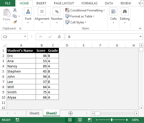
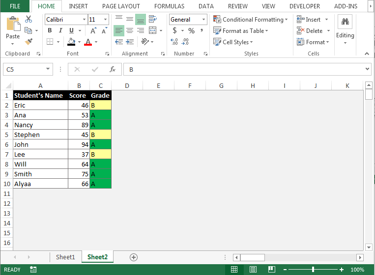
We have data in range A1:C10 in which Column A contains Student’s name, column B contains Scores and in column C is having grades. We need to highlight grades with color such as “A” grade with green color and “B” grade with blue color.

To color rows based on text criteria:

Select the range C2:C10 by pressing the key “CTRL+SHIT+Down arrow key”.
Go to the “Home Tab” and then in the “Styles” group select “New Rule” from the Conditional Formatting dropdown menu.
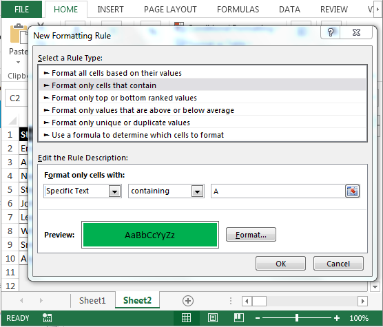
The “New Formatting Rule” dialog box will appear.
Select the rule type “Format only cells that contain”. In the “Edit the Rule Description” select “Specific Text” from the dropdown menu.
In 2^nd dropdown menu, select “Containing”, type “A” in the box.
In the dialog box below you will see the “Format” option. Click on the “Format” icon, the “Format Cells” dialog box will be active. . In the “Fill” tab, select the green color and click on OK.
The selected color will be displayed in the “Preview” box and then click on OK.

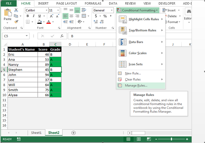
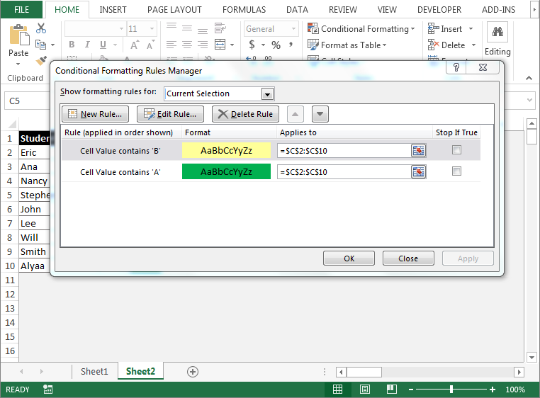
Now select “Manage Rule” from the drop menu of “Conditional Formatting”.

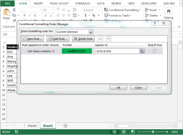
The “Conditional Formatting Rules Manager” dialog box will appear.

Click on “New Rule”, and the “New Formatting Rule” dialog box will get activated.
Select a rule type “Format only cells that contain”. In the “Edit the Rule Description” box select “Specific Text” from the dropdown menu.
In the 2^nd dropdown menu, select “Containing”, type “B” in the box.
In the dialog box below the “Format” option is shown. Click on the “Format” icon, the “Format Cells” dialog box will get activated. In the “Fill” tab, select the yellow color and click on OK.
In the “Conditional Formatting Rules Manager” dialog box, click on apply, then click on OK.