Retrieving the Closest Larger and Smaller Values from a List in Microsoft Excel

In Excel if you have a list of values and you cannot find an exact match, then you need to find either the Closest Larger or Closest Smaller value. For example, if you are doing a comparison of numbers and you do not find an exact match in the range, you can use the next larger or smaller number and proceed ahead.

We can use a combination of the Countif, Large and Small formula to get our output.

Countif is used to count the number of times specific data is repeated in a range of cells.

Syntax =COUNTIF(range,criteria)

Large: Returns the k-th largest value in a data set.

Syntax =LARGE(array,k)

Small: Returns the k-th smallest value in a data set.

Syntax =SMALL(array,k)

Let us understand what is Closest Larger & Smaller Number

We have a list with random numbers 1,2,3,5,8,10 and we need a formula to evaluate the following:

-         If k is in the list, return k

-         If k is not in the list, return the next higher value. For example, if k =7, return 8 (in case of closest larger number)

-         If k is not in the list, return the next smaller value. For example, if k =7, return 5

(in case of closest smaller number)

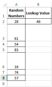
Let’s take an example, we have some random numbers in column A & we need to find the value in this range, which is the Closest Smaller or Closest Larger to cell B2 which contains 46. This number is not available in our range.  See the below screenshot

Let us see how we calculate the Closest Larger Number first:

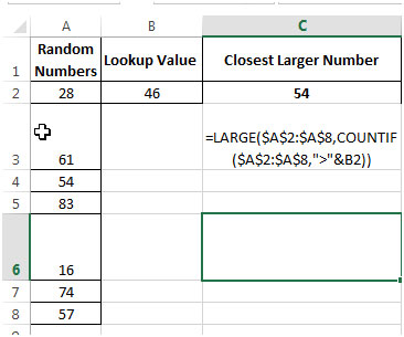
We can manually check the next largest value to 46 which is 54.

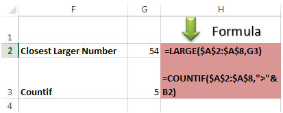
Now lets try to obtain the same result using formula -

• We will use a combination of the LARGE & COUNTIF functions to generate the closest larger number.
• Criteria is greater than ‘>’ sign with Lookup Value i.e. cell B2
• The greater than sign combined with the Lookup value will return 5 values i.e. 54, 57, 61, 74, 83 which are larger than 46.
• When we merge theLarge &Countiffunctions, we will get 54.  Refer to the formula in cells G2 and G3 in the snapshot below.

PS: B2 in Countifformula is the Lookup Value i.e. 46

• In cell C2, the formula used for finding Closest Larger number is    =LARGE($A$2:$A$8,COUNTIF($A$2:$A$8,">"&B2))

Now let us see how we calculate the Closest Smaller Number -

We can manually check the next smaller value to 46 which is 28.

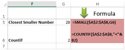
Lets obtain the same output using formula -

• We will use a combination of the SMALL& COUNTIFfunctions to generate the closest smaller number.
• Criteria is lessthan ‘<’ with Lookup Value i.e. cell B2
• Less than sign combined with the Lookup value will return 2 values, i.e.16& 28which are smaller than 46.
• When we merge the Small &Countiffunctions, we get 28. Refer to the formula in cells G5 and G6 in the snapshot below.

See below screenshot with formula:

Note: cell B2 in CountifFormula is the Lookup Value i.e. 46

• In cell D2, the Formula used for finding Closest Smaller number is  =SMALL($A$2:$A$8,COUNTIF($A$2:$A$8,"<"&B2))

This is the how we can return the closest larger number and closet smaller number.