To save the criteria while filtering data,, you need to use Custom View in Microsoft Excel.
What is Custom View?
This tool is used to save the current display and print settings as a custom view that you can quickly apply in the future.
Let’s take an example and understand how we can save the filtering criteria -.
Add the “Custom View” icon to the toolbar.

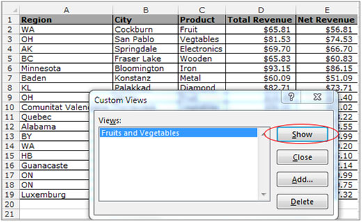
I have data in range A1:E19. In which column A contains the “Region”, column B “City”, column C “Product”, column D “Total Revenue” and column E contains “Net Revenue”.
Save the Filtering criteria


To check the “Custom Views” follow the below mentioned steps:-


If you liked our blogs, share it with your friends on Facebook. And also you can follow us on Twitter and Facebook.
We would love to hear from you, do let us know how we can improve, complement or innovate our work and make it better for you. Write us at info@exceltip.com
The applications/code on this site are distributed as is and without warranties or liability. In no event shall the owner of the copyrights, or the authors of the applications/code be liable for any loss of profit, any problems or any damage resulting from the use or evaluation of the applications/code.
Thanks a ton. I have been looking for this one since long. Finally, something for my rescue.
-Subhas
Hi Jazz,
When you save the data with filter then you can copy data and paste into new worksheet and then send to the recipient .
Imran.
If I save a worksheet with filters applied to a column, and send it to someone, say via email, the recepient will by default see the worksheet with filtered content, but then can remove the filter and see the entire content. What I want to do is: the worksheet should be saved only with the filtered data, and the rest of the data is deleted. Is there any way to do that?
Jazz
(PS: I am only a beginner, so please be in detail. Thanks)
THANKS A LOT
My document has over 632,000 rows, and probably 15 columns that contains data for the entire U.S. I am trying to filter by individuals states, which I can do.....BUT, when I try to save that filtered document (to save by the states I need)it does not work. It saves the entire document again. Even if you simply highlight it will not save. Can you help me please? Thanks
"Hi Pedro,
There might be an easy way around that, but I don't know it.
I guess you could write VBA code to do this though. It would have to unprotect, select the custom view, and then re-protect.
Note that *sheet protection* is only ever a nominal security even with a password - they are trivial to break, so you could 'hide' the password in the VBA code working on the assumption that anyone who knows how to read VBA code will also be able to break the sheet protection if they wanted to.
HTH,
Alan."
"Hello Alan,
Thanks but No, Thanks...
The worksheet is supposed to be protected so the user won't mess around with protected fields...but still it would be handy to have those views ready for printing purposes. By the way, the custom views list doesn't come alphabetically sorted. Is there anyway to sort it ?
Thanks in advance
Regards
Pedro Bonniz"
"Hi Pedro,
Why not just un-protect the worksheet?
Alan."
"Hi Bill,
MATCH or one of the LOOKUP functions should work fine.
How is it not working for you specifically?
Alan."
Unfortunately, Custom Views won't work while the worksheet is protected. The message "Some view settings could not be applied." will pop up and it just doesn't work..., or doesl it ?
I work in the auto parts business & I constantly have to check inventories. Here is what I need to do: I have a column of numbers for example 1,2,3,4,5,6. I need to input another colum of numbers, example, 1,4,5 and have them "match up" with the 1st column. I have tried "match" and just can't seem to get it to work. This would really help me greatly. Thanks in advance