In this article, we will learn how to how to calculate cumulative principal payment using Excel CUMPRINC formula.
Scenario :
When working with loan amount and its related queries. Sometimes we need to know how much loan amount or principal amount is paid over a given period of time. Every installment includes part of principal amount and tax amount. This formula returns the part of principal amount paid between given start and end time.
CUMPRINC function in Excel
The CUMPRINC function calculates the portion of principal amount for a cumulative loan based on terms over a given period of time in Excel.
Generic Formula:
rate – The interest rate per period.
nper – The total number of payments.
pv – the loan amount
Start - start month for the period
end period - end month for the period
Type – The timing of the payment, either at the beginning or end of the period. Numbers 0 or 1 represent the payment date. The number 0 represents payment at the end of the period, and the number 1 represents payment at the beginning of the period. The default (empty argument) is 0. The calculation is at the end of the period.
EXAMPLE:
All of the above might be confusing for some people, so let’s gear up & start learning its usage in excel with the example.
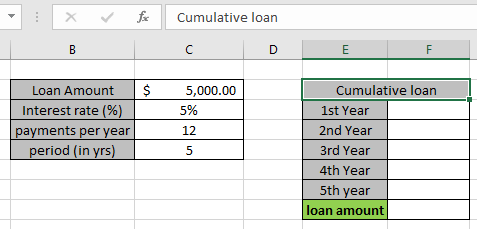
Consider a scenario where John has taken a loan of $5,000 from a bank at 5% interest rate per year over a 5 years period. He needs to find out how much principle loan amount he is paying every year. First we will calculate the principal loan amount for the first year and then we will calculate the amount of later years. The sum of total amount of all years must be equal to the total loan amount which is $5,000.
So he added the following terms on loan in Excel.

So with given details we can find out the cumulative loan for the first year
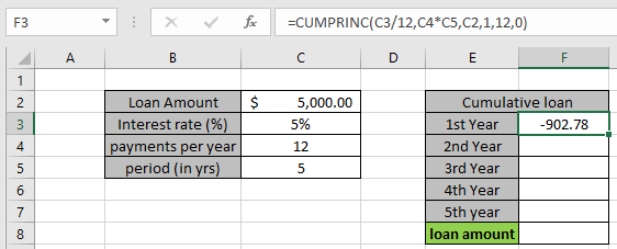
Use the formula in F3 cell
Explanation:
C3/12 : rate value is divided by 12 as the payment made every year are 12.
C4*C5 : nper, total payment made for the loan. Payment made in an year * total years.
C2 : pv, present value of the loan or the loan amount
1 , 12 : start and end period for the first year cumulative loan.
0 : payment at the end of the period

The formula in the cell is like as shown in the snapshot above. Arguments to the function are given in as using cell reference.

John paid $ 902.78 for the first year. You must be wondering why this amount shown here is negative. The loan amount is positive which is credited to John. He has to pay that amount which is to be debited.
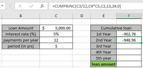
To find the cumulative loan for the Second year, the start and end period be defined as follows:
Start period : 13
End period : 24
Use the formula in F4 cell:

John paid $ 948.96 for the second year.
To find the cumulative loan for the Third year, the start and end period be defined as follows:
Start period : 25
End period : 36
Use the formula in F4 cell:

John paid $ 997.51 for the third year.
To find the cumulative loan for the Fourth year, the start and end period be defined as follows:
Start period : 37
End period : 48
Use the formula in F4 cell:

John paid $ 1048.55 for the Fourth year.
To find the cumulative loan for the fifth year, the start and end period be defined as follows:
Start period : 49
End period : 60
Use the formula in F4 cell:

John paid $ 1,102.20 for the Fifth year. As calculating the sum of all years will be equal to the total loan amount $5000.
Here are some observational notes shown below.
Notes:
Hope you understood how to calculate cumulative loan using CUMPRINC function in Excel. Explore more articles here on calculating accounts function here.
If you liked our blogs, share it with your friends on Facebook. And also you can follow us on Twitter and Facebook. We would love to hear from you, do let us know how we can improve, complement or innovate our work and make it better for you. Write us at info@exceltip.com
Related Articles
How to Use PV function in Excel
How to Use NPV function in Excel
How to Use FV function in Excel
How to use the IPMT Function in Excel
Simple interest formula in Excel
How to calculate interest on a loan
How to use XNPV function in Excel
How to Use RATE Function in Excel
Popular Articles
50 Excel Shortcut to Increase Your Productivity
If with conditional formatting
The applications/code on this site are distributed as is and without warranties or liability. In no event shall the owner of the copyrights, or the authors of the applications/code be liable for any loss of profit, any problems or any damage resulting from the use or evaluation of the applications/code.