In this article, we will learn about how to use the DDB function in Excel.
DDB function is rate or factor declining depreciation is the way of calculating the different depreciation of any asset for each period. Double declining balance method is the way where user can add a factor or rate of decline of depreciation of an asset for a specific period.
The DDB function returns depreciation decline amount by a factor or rate for the input data for the specific product.
Syntax:
Cost : Cost price of the asset
Salvage : remaining price of the asset after its lifetime period
Life : period after which cost price becomes salvage price
period : specific period for which we need to calculate depreciation.
factor : [optional] specify rate or factor for the asset depreciation. Default is 2
Let’s understand this function using it in an example.
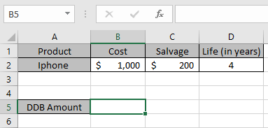
Here we took a product as Iphone. The cost price & salvage price of the latest Iphone is shown in the snapshot below.

Now we need to calculate the depreciation amount for the Iphone by factor 1.
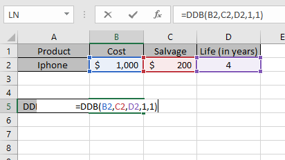
Use the formula to calculate depreciation by factor 1:
B2 : Cost price of the asset
C2 : remaining price of the asset after a period
D2 : 4 years after cost price becomes salvage price
1 : first year to calculate depreciation amount.
1 : via factor

The values to the formula are taken as cell reference.

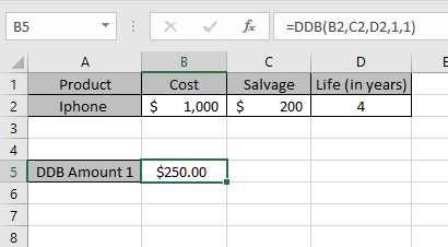
As you can see from the above returned value, first year $ 250 will depreciated from the asset cost value.
Now we will calculate the depreciation amount for each year separately and for different factors.
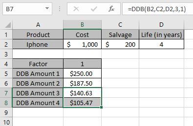
Use the formula to calculate depreciation for second year:
B2 : Cost price of the asset
C2 : remaining price of the asset after a period
D2 : 4 years after cost price becomes salvage price
2 : first year to calculate depreciation amount.
1 : via factor
Month : taken as default to 12 a year.

Similarly calculate the depreciation for Third & Fourth year

So, we got different depreciation for each period via factor 1.
Now we will get the depreciation values varying factors

| Factor | 1 | 2 | 3 |
| DDB Amount 1 | $250.00 | $500.00 | $750.00 |
| DDB Amount 2 | $187.50 | $250.00 | $50.00 |
| DDB Amount 3 | $140.63 | $50.00 | $0.00 |
| DDB Amount 4 | $105.47 | $0.00 | $0.00 |
This is the drop depreciation table for the asset varying factors of 1, 2 & 3
DDB function shows that depreciation reduces as factor value increases.
You can see from the above table that depreciation amount is deducted from the salvage amount for every year up till life of an asset.
Note:
Hope you understood how to use DDB function and referring cell in Excel. Explore more articles on Excel financial functions here. Please feel free to state your query or feedback for the above article.
Related Articles
How to use the VDB Function in Excel
How to use the DB Function in Excel
How to use the SYD Function in Excel
Popular Articles:
50 Excel Shortcuts to Increase Your Productivity
How to use the VLOOKUP Function in Excel
The applications/code on this site are distributed as is and without warranties or liability. In no event shall the owner of the copyrights, or the authors of the applications/code be liable for any loss of profit, any problems or any damage resulting from the use or evaluation of the applications/code.