In this article, we will learn how to color unique record in a range. We use the Conditional Formatting option along with COUNTIF function in Microsoft Excel to get the desired outcome.
Conditional Formatting we use to highlight the important points with color in a report.
COUNTIF function we use to count how many times one word is appearing in a column.
Let’s take an example to understand how we can highlight the unique cells.
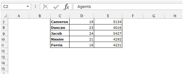
We have data in range C2:E11 in which column C contains Agents name, column D contains No. of sales and column E contains sales amount. Now, we want to highlight the unique Agents name with the color.

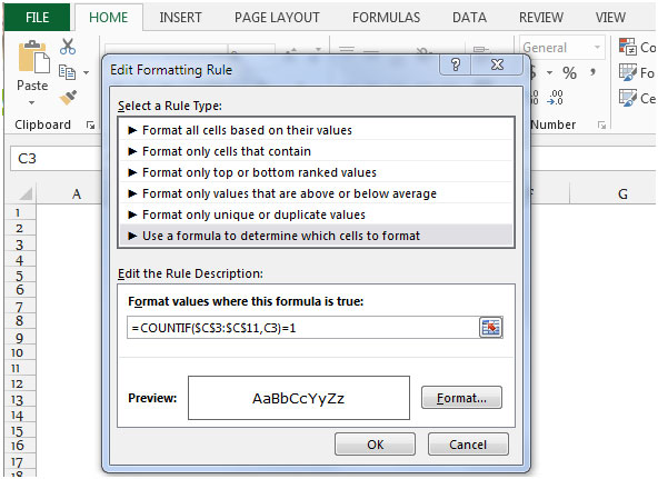
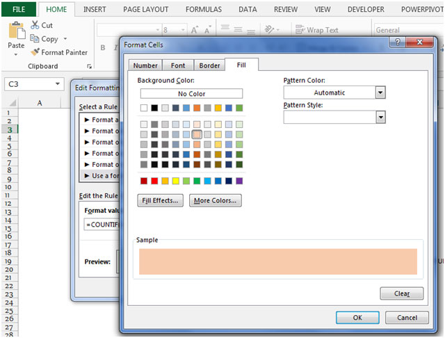
To highlight the Unique Agents name, follow the below given steps:-


All unique cells will get highlighted with the chosen color. This is the way we can highlight the unique text in a range by using the Conditional Formatting option along with COUNTIF function.
If you liked our blogs, share it with your friends on Facebook. And also you can follow us on Twitter and Facebook.
We would love to hear from you, do let us know how we can improve, complement or innovate our work and make it better for you. Write us at info@exceltip.com
The applications/code on this site are distributed as is and without warranties or liability. In no event shall the owner of the copyrights, or the authors of the applications/code be liable for any loss of profit, any problems or any damage resulting from the use or evaluation of the applications/code.