
In this article, we will learn how to use shrink to fit option to adjust text in cells in Excel.
Scenario:
Whenever working with data, we always receive data in an untidy manner. So first we need to clean data via editing cells to make it presentable. So this article helps you to shrink long text data in cells. Below is the detailed understanding of the shrink to text option.
How to solve the problem?
Here we will follow a process which will help you understand how Excel interprets long text data in cell. Usually excel cells spill the text over to the next cell when the length of string is more than the length of the cell. But if the adjacent cell is occupied, then either the exceeded text is hidden or the cell shows #####. So we can just select the whole column and double click on the right side of the column as shown below.

Here in the above gif, it shows a table where the G column length is extended to the limit of the longest string in the column. Below is the detailed understanding of shrink to fit option and other options used along with this option.
Example :
All of these might be confusing to understand. So let's take a sample of untidy data and clean it step by step and at last you will understand how a cell interprets data in excel.

Here we have a sample of data of customers who bought products from a superstore. Now the manager wants to see the data to verify numbers, but he receives this data. The data has some spilled over text, some ##### values. So, for this we will follow a process explained below to clean data including shrink to fit option. Here we in the process we will fix row and column size of the data.
Select the data and use the centre align option to align all text to centre vertically and horizontally.
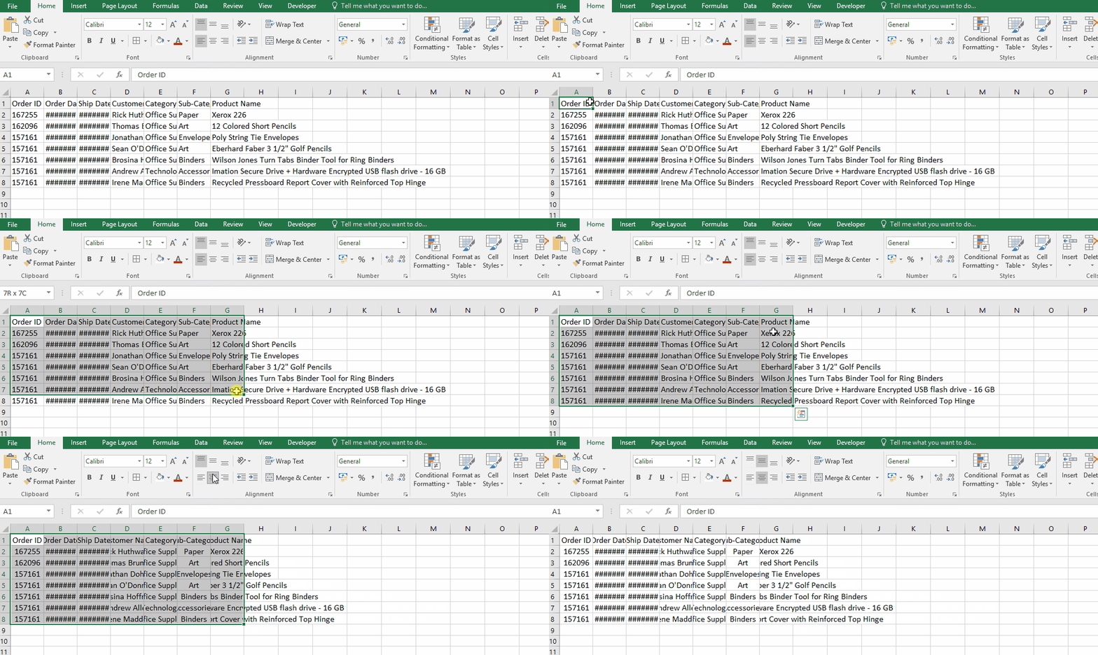
Now we select the small triangle on the top left of data and double click the column gap and row gap, which adjusts cell length according to the largest length in a particular column as shown below.
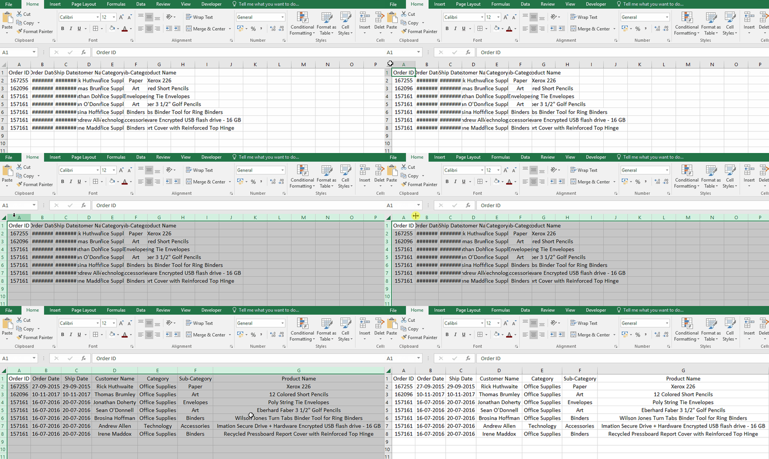
As you can see from the above gif, all values are visible and centre aligned.
Now we fix an average length of all rows in data. Select the rows from the numbers on the left side and then use right click -> Row height -> fix length to 30.

As you can see, the length of rows are extended. Follow the same process for the required columns only as shown below. Here the required column in the G column.

Now we fixed the length of the cells. Now we select the whole data again -> right click -> select Format cells from the drop down list as shown below.

Format cell dialog box appears, now select the Alignment tab. The box will appear as shown below.
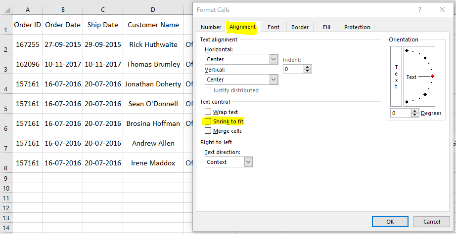
Select the option Shrink to fit option, If this option is disabled. Then first deselect the wrap text and then select the Shrink to fit as shown below.

The table will be shown like as shown below.
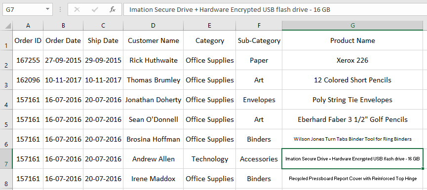
As you can see in the table from the above image, the longer text values shrink to fit. As you edit the value, the text length will be changed automatically. You can also use the wrap text option to wrap strings in lines in the same cell as explained below.
Select the data and click wrap text from the format cell dialog box or wrap text option on the front panel.
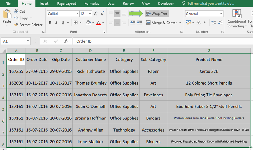
Now click the option and the table values will shrink by wrapping text into different lines as shown below.

Now you can do these steps in any manner as it doesn't affect or edit any cell. This process is used to shrink values in data by either varying the font size of the value or wrapping text in different lines. You can vary the length row and column by just dragging the end limit to required length.
Hope this article about How to shrink to fit text option in Excel cell is explanatory. Find more articles on text formulas here. If you liked our blogs, share it with your fristarts on Facebook. And also you can follow us on Twitter and Facebook. We would love to hear from you, do let us know how we can improve, complement or innovate our work and make it better for you. Write us at info@exceltip.com
Related Articles:
50 Excel Shortcut’s to Increase Your Productivity : The Excel shortcuts enhance the efficiency of work a lot. These 50 shortcuts can increase your productivity exceptionally on Excel
Excel Insert Row Shortcut : These shortcuts will help you insert single and multiple rows quickly.
Excel Shortcut Keys for Merge and Center : This Merge and Center shortcut helps you quickly merge and unmerge cells.
Replace text from end of a string starting from variable position : To replace text from the end of the string, we use the REPLACE function. The REPLACE function use the position of text in the string to replace.
How to Select Entire Column and Row Using Keyboard Shortcuts in Excel : Selecting cells is a very common function in Excel. Use Ctrl + Space to select columns and Shift + Space to select rows in Excel.
Popular Articles:
How to use the IF Function in Excel : The IF statement in Excel checks the condition and returns a specific value if the condition is TRUE or returns another specific value if FALSE.
How to use the VLOOKUP Function in Exceln : This is one of the most used and popular functions of excel that is used to lookup value from different ranges and sheets.
How to use the COUNTIF Function in Excel : Count values with conditions using this amazing function. You don't need to filter your data to count specific values. Countif function is essential to prepare your dashboard.
How to use the SUMIF Function in Excel : This is another dashboard essential function. This helps you sum up values on specific conditions.
The applications/code on this site are distributed as is and without warranties or liability. In no event shall the owner of the copyrights, or the authors of the applications/code be liable for any loss of profit, any problems or any damage resulting from the use or evaluation of the applications/code.