A good database is always structured. It means different entities have different tables. Although, Excel is not a database tool but is often used to maintain small chunks of data.
Many times we get the need of merging tables in order too see a relationship and churn out some useful information.
In databases like SQL, Oracle, Microsoft Access, etc, it is easy to join tables using simple queries. But in excel we don't have JOINs but we can still join tables in excel. We use Excel Functions to merge and join data tables. Perhaps it is a more customizable merge than SQL. Let’s see the techniques of merging excel tables.
To merge data in excel, we should have at least one common factor/id in both tables, so that we can use it as a relation and merge those tables.
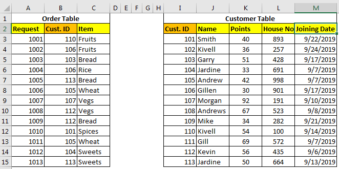
Consider these two tables below. How can we combine these data tables in Excel?

The Order Table has order details and the Customer table contains customer details. We need to prepare a table that tells which order belongs to which customer name, customer’s points, house number, and his joining date.
The common id in both tables is Cust.ID which can be used for merging tables in excel.
There are three methods of merging tables using VLOOKUP Function.
Retrieve Each Column With Column Index
In this method, we will use simple VLOOKUP to add these tables in one table. So to retrieve name write this formula.
[Customers is Sheet1!$I$3:$M$15.]
To merge points in table, write this formula.
To merge house no in table, write this formula.

Here we merged two tables in excel, each column one by one in the table. This is useful when you have only few columns to merge. But when you have multiple columns to merge, this is can be a hectic task. So to merge multiple tables we have different approaches.
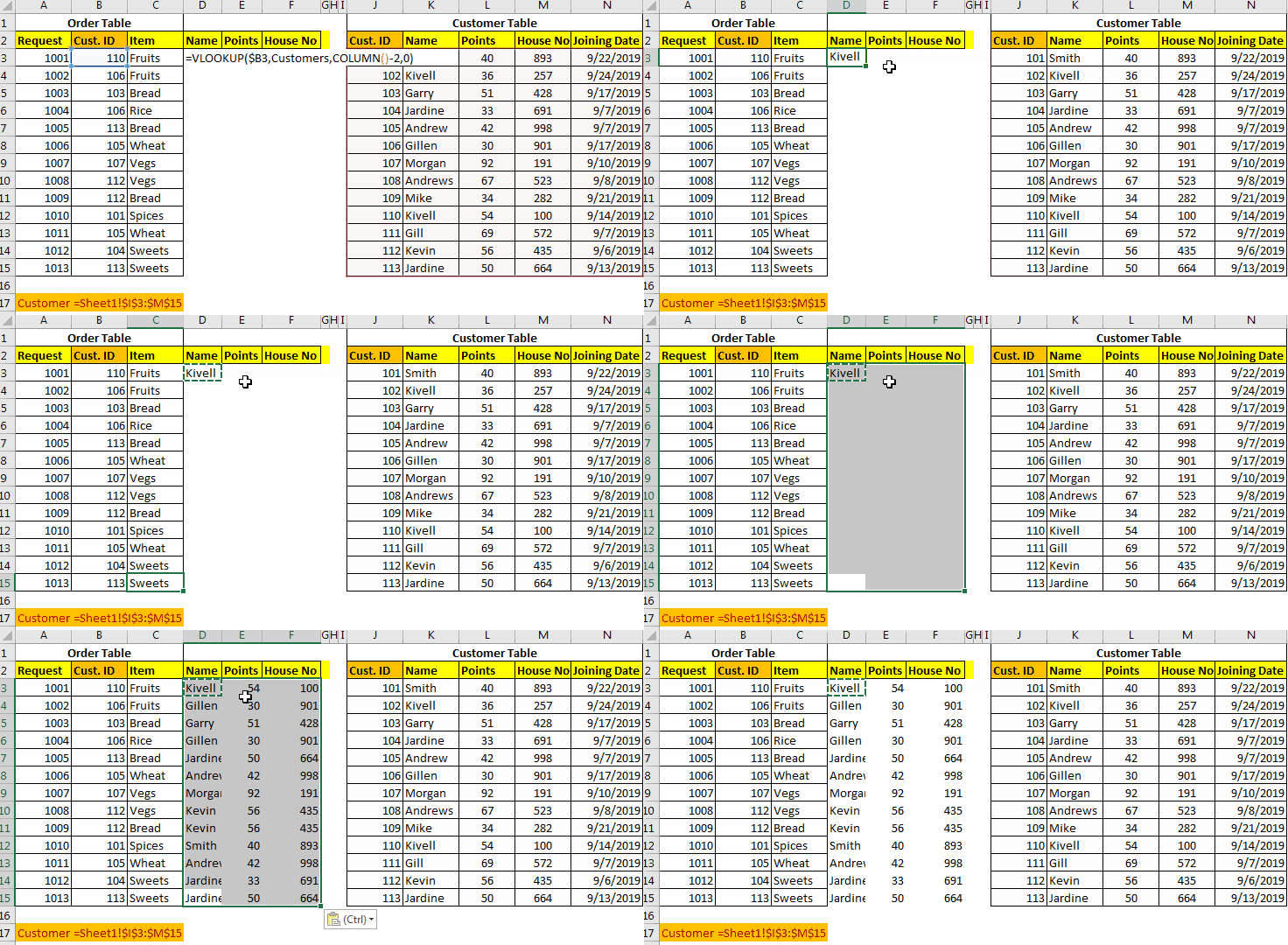
When you want to retrieve multiple adjacent columns, use this formula.
Here the COLUMN function just returns the column numbers in which the formula is being written.
n is any number which adjusts the column number in table array,
In our example, the formula for table merging will be:
Once you write this formula, you will not have to write the formula again for other columns. Just copy it in all other cells and columns.

How It Works
Ok! In the first column, we need a name, which is the second column in customer table.
Here the main factor is COLUMN()-2. The COLUMN function returns the column number of current cell. We are writing the formula in D3, hence we will get 4 from COLUMN(). Then we are subtracting 2 which makes 2. Hence finally our formula simplifies to =VLOOKUP($B3,Customers,2,0).
When we copy this formula in E columns we will get the formula as =VLOOKUP($B3,Customers,3,0). Which retrieves 3rd column from customer table.
Merge Tables Using VLOOKUP-MATCH Function
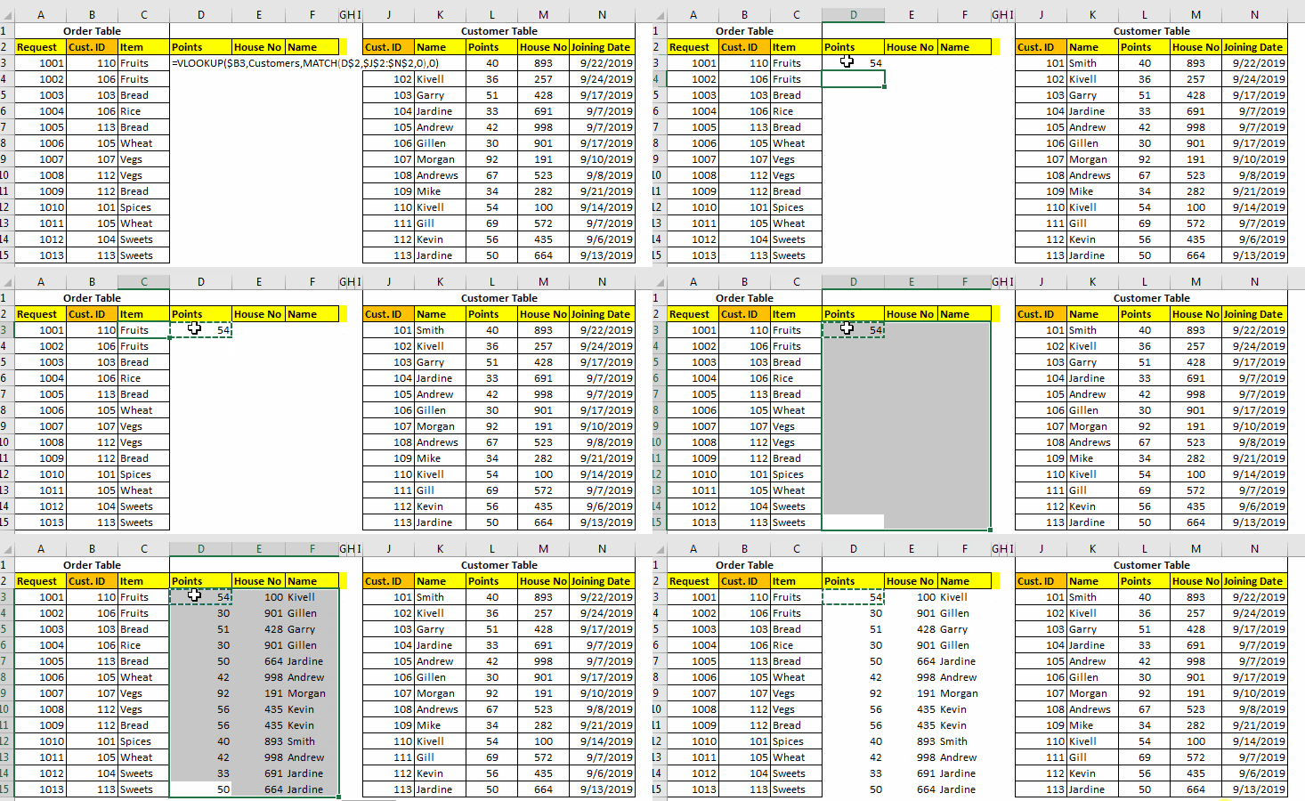
This one is my favorite way of merging tables in excel using the VLOOKUP function. In the above example, we retrieved column in serial. But what if we had to retrieve random columns. In that case above Techniques will be useless. The VLOOKUP-MATCH technique uses column headings to merge cells. This is also called VLOOKUP with Dynamic Col Index.
For our example here, the formula will be this.

Here, we are simply using MATCH function to get the appropriate column number. This called Dynamic VLOOKUP.
Using INDEX-MATCH to Table Merging in Excel
The INDEX-MATCH is very powerful lookup tool and many time it is referred as better VLOOKUP function. You can use this to for combining two or more tables. This will also allow you to merge columns from left of the table.
This was a quick tutorial about merging and joining tables in excel. We explored several ways of merging two or more tables in excels. Feel free to ask question about this article or any other query regarding excel 2019, 2016, 2013 or 2010 in the comments section below.
Related Articles:
IF, ISNA and VLOOKUP function in Excel
IFERROR and VLOOKUP function in Excel
How to retrieve the entire row of a matched value in Excel
Popular Articles :
50 Excel Shortcut to Increase Your Productivity : Get faster at your task. These 50 shortcuts will make you work even faster on Excel.
How to use the VLOOKUP Function in Excel : This is one of the most used and popular functions of excel that is used to lookup value from different ranges and sheets.
How to use the COUNTIF function in Excel : Count values with conditions using this amazing function. You don't need to filter your data to count specific values. Countif function is essential to prepare your dashboard.
How to use the SUMIF Function in Excel : This is another dashboard essential function. This helps you sum up values on specific conditions.
The applications/code on this site are distributed as is and without warranties or liability. In no event shall the owner of the copyrights, or the authors of the applications/code be liable for any loss of profit, any problems or any damage resulting from the use or evaluation of the applications/code.