How to use the BITLSHIFT Function in Excel

IN this article, we will understand How to use the BITLSHIFT Function in Excel

Scenario:

This function was introduced in Excel 2013 and it returns a number shifted left by bits specified as numbers. For example, binary representation of 8 is 1000 and adding two 0 digits on the right of it will make it as 100000, which is number 32 in decimal.

The BITLSHIFT function in excel performs the Bitwise Left Shift operation on a decimal number and returns the decimal number after the operation is performed. Bitwise left shift operation is performed on a binary number. Let’s consider a decimal number 4 and a bit left shift to be 2. As we know 4 is represented as 100 in binary. So 2 zeros will be added to the right of the binary number by shifting left.

BITLSHIFT function

The BITLSHIFT function returns a Bitwise Left Shift of a decimal number upto shift_amount.

Syntax:

number1 : a positive integer number of base 10 (decimal number) to be shifted

shift_amount : an integer representing the amount of shift to occur on the number. This argument can be positive , zero or negative.

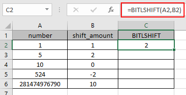
Here is the excel representation of the function

As you can the function returns 16 after the bitwise left shift of 2 on 4.

You can use the DEC2BIN & BIN2DEC function in excel to understand the conversion operation.

Now let’s get more understanding of the function via using them in some examples.

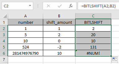
Here we have some values as number & shift_amount in Columns. We need to get the bitwise left shift operation on the given numbers using the BITLSHIFT function in excel

Use the formula :

A2 : number provided to the function as cell reference

B2 : number provided to the function as cell reference

The bitwise left shift operation on 1 ( 01 ) by adding one zero to the right of the number will be 2 ( 010 ).

Now copy the formula to other cells using the Ctrl + D shortcut key.

As you can see here the BITLSHIFT function returns the result of the input values.

Notes:

1. Numbers can be given as argument to the function directly or using the cell reference in excel.
2. The numbers must be a valid decimal number between 0 & 281474976710655.
3. If a negative number is provided as Shift_amount argument to the function, the value shifts right.
4. If Number is greater than (2^48)-1, you will get #NUM! error and you'll get #VALUE! error if either of the above two arguments is a non - numeric value.
5. The function returns the #NUM! Error
   1. If either of the decimal number is less than 0 or greater than 281474976710655 which is 248-1.
   2. If the resulting number exceeds the range of 0 to 248-1.
6. The function returns the #VALUE! Error,
   1. If the input number is text or non-numeric.
   2. If the shift_amount argument is text or non numeric.
   3. If the shift amount is less than -53 or greater than + 53.

Related Articles :

How to use the BITLSHIFT Function in Excel : BITLSHIFT function in excel performs the Bitwise Left Shift operation on a decimal number and returns the decimal number after the operation performed.

How to use the BITRSHIFT Function in Excel : BITRSHIFT function in excel perform the Bitwise Right Shift operation on a decimal number and returns the decimal number after the operation performed.

How to use the HARMEAN Function in Excel : Harmonic mean of n numbers (a ,b ,c ,d , . . .) in mathematics is calculated using the HARMEAN function in Excel.
How to use the BITOR Function in Excel : BITOR function in excel perform the Bitwise OR operation between the two decimal numbers and returns the decimal number after the operation performed.

How to use the BITAND Function in Excel : BITAND function in excel perform the bitwise AND operation between the two decimal numbers and returns the decimal number after the operation performed.

Popular Articles :

50 Excel Shortcuts to Increase Your Productivity : Get faster at your task. These 50 shortcuts will make you work even faster on Excel.

How to use the IF Function in Excel : The IF statement in Excel checks the condition and returns a specific value if the condition is TRUE or returns another specific value if FALSE.

How to use the VLOOKUP Function in Excel : This is one of the most used and popular functions of excel that is used to lookup value from different ranges and sheets.

How to use the SUMIF Function in Excel : This is another dashboard essential function. This helps you sum up values on specific conditions.

How to use the COUNTIF Function in Excel : Count values with conditions using this amazing function. You don't need to filter your data to count specific values. Countif function is essential to prepare your dashboard.