In this article, we will learn about how to use the BITXOR function in Excel.
Scenario:
BITXOR function in excel perform the BITWISE XOR operation between the two decimal numbers and returns the decimal number after the operation performed.
XOR operation is a logical operator used in communication processes. AND operator is performed over the 2 bits ( 0 or 1 ). The operation takes place like in table shown below.
| Bit 1 | Bit 2 | AND operation |
| 0 | 0 | 0 |
| 0 | 1 | 1 |
| 1 | 0 | 1 |
| 1 | 1 | 0 |
Here the decimal numbers be changed in binary and the OR operation be performed over each bit with the corresponding bits.
| Decimal | Binary | |
| number1 | 2 | 010 |
| number2 | 4 | 100 |
| result | 6 | 110 |
The different highlighted bits is to show how the BITWISE XOR operation occurs between the two numbers. Use the DEC2BIN function ( decimal to binary conversion) & BIN2DEC function ( binary to decimal conversion) to understand BITXOR function’s result step by step in Excel. For example, Binary representation of 10 is 1010 and Binary representation of 7 is 111 and if we compare which positions are not equal we will get :-
1010
0111
-------
yyny
4301
so that means 1*(2^3)+1*(2^2)+1*(2^0) = 8+4+1=13
so if we use the formula directly as =BITXOR(10,7) will get the similar result as 13.
BITXOR function
The BITXOR function returns a bitwise 'XOR' of two numbers.
Syntax:
| =BITXOR ( number1, number2) |
number1 : a positive integer number of base 10 (decimal number).
number2 : a positive integer number of base 10 (decimal number).
Example :
All of these might be confusing to understand. Let's understand how to use the function using an example. Here is the excel representation of the function. The below image shows the result in B4 cell taking input B2 and B3 cell.
Use the formula :
| =BITXOR (B2, B3) |

As you can see, the Bitxor operation of 2 and 10 returns 8.
Now let’s get more understanding of the function via using them in some examples.

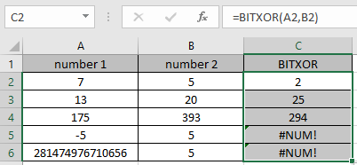
Here we have some values as number1 & number 2 in Columns. We need to get the Bitwise 'XOR' operation on the given numbers
Use the formula :
| =BITXOR (A2, B2) |
A2 : number provided to the function as cell reference
B2 : number provided to the function as cell reference

The Bitwise 'XOR' operation on 7 ( 111 ) & 5 ( 101 ). Resulting binary number would be 101. So the decimal number representing 101 is 5.
Now copy the formula to other cells using the Ctrl + D shortcut key.

As you can see here the BITXOR function returns the result of the input values.
Here are some observational notes using the BITXOR function in Excel.
Notes :
Hope this article about how to use the BITXOR function and referring cell in Excel is explanatory. Find more articles on Bit wise formulas and related Excel formulas here. If you liked our blogs, share it with your friends on Facebook. And also you can follow us on Twitter and Facebook. We would love to hear from you, do let us know how we can improve, complement or innovate our work and make it better for you. Write to us at info@exceltip.com.
Related Articles :
How to use the BITLSHIFT Function in Excel : BITLSHIFT function in excel performs the Bitwise Left Shift operation on a decimal number and returns the decimal number after the operation performed.
How to use the BITRSHIFT Function in Excel : BITRSHIFT function in excel perform the Bitwise Right Shift operation on a decimal number and returns the decimal number after the operation performed.
How to use the HARMEAN Function in Excel : Harmonic mean of n numbers (a ,b ,c ,d , . . .) in mathematics is calculated using the HARMEAN function in Excel.
How to use the BITOR Function in Excel :
How to use the BITAND Function in Excel :
Popular Articles :
How to use the IF Function in Excel : The IF statement in Excel checks the condition and returns a specific value if the condition is TRUE or returns another specific value if FALSE.
How to use the VLOOKUP Function in Excel : This is one of the most used and popular functions of excel that is used to lookup value from different ranges and sheets.
How to Use SUMIF Function in Excel : This is another dashboard essential function. This helps you sum up values on specific conditions.
How to use the COUNTIF Function in Excel : Count values with conditions using this amazing function. You don't need to filter your data to count specific values. Countif function is essential to prepare your dashboard.
The applications/code on this site are distributed as is and without warranties or liability. In no event shall the owner of the copyrights, or the authors of the applications/code be liable for any loss of profit, any problems or any damage resulting from the use or evaluation of the applications/code.