In this article, we will learn How to use the ADDRESS function in Excel.
ADDRESS of cell reference
Whenever you need to access the address of the cell having some criteria. You won't be using it till long. You can use the ADDRESS function. Let's understand the ADDRESS function syntax and illustrate the ADDRESS function usage with an example.
ADDRESS Function in Excel
The ADDRESS function simply returns the address of a cell by using row number and column number.
ADDRESS Function syntax :
| =ADDRESS(row_num,col_num,[abs_num],[a1],[sheet_name]) |
Row_num: The Row number
Col_num: The Column number
[abs_num]: Optional Argument. Has four possible inputs, 1, 2, 3, and 4. If omitted or 1, the returned address will be absolute eg $A$1. 2 returns absolute row and relative column eg A$1.
3 returns relative row and absolute column $A1. 4 returns relative address eg A1.
[a1]: Optional Argument. Has two possible inputs, 0 and 1. If omitted, it will return A1-style. 0 returns output in R[1]C[1] style.
[sheet_name]: Optional Argument. If a sheet name is provided, add it with the address along ! mark. Eg. mysheet!A1.
IMPORTANT: The address returned is in text format.
Example :
All of these might be confusing to understand. Let's understand how to use the function using an example.
| =ADDRESS(3,1,4) |
Above ADDRESS formula will return A3.
| =INDIRECT(ADDRESS(3,1)) |
Above formula will return value at $A$3
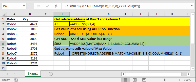
We have this table.

Write this formula anywhere to get address of Max Value.
| =ADDRESS(MATCH(MAX(B:B),B:B,0),COLUMN(B2)) |
MAX function finds max value in range B:B
MATCH looks for that MAX value in B:B range and returns index or say row number.
COLUMN returns column number of B2.
Now, ADDRESS has row_num and col_num. And this is all it needs.
Many times you would require to get the name of a person getting max or min value. One approach is this.
| =OFFSET(INDIRECT(ADDRESS(MATCH(MAX(B:B),B:B,0),COLUMN(B2))),0,-1) |
Since address returned by ADDRESS function is text, we use INDIRECT so that OFFSET function takes it as real address.
we move 1 column left to max cell using -1. And finally offset returns name of robo that is getting max pay.
Here are all the observational notes using the ADDRESS function in Excel
Notes :
Hope this article about How to use the ADDRESS function in Excel is explanatory. Find more articles on calculating values and related Excel formulas here. If you liked our blogs, share it with your friends on Facebook. And also you can follow us on Twitter and Facebook. We would love to hear from you, do let us know how we can improve, complement or innovate our work and make it better for you. Write to us at info@exceltip.com.
Related Articles :
How to use the CELL function in Excel : returns information about a cell in a worksheet using the CELL function.
How to use the TYPE Function in Excel : returns numeric code representing the TYPE of data using TYPE function in Excel.
How to use the SHEETS function in Excel : returns a number, reference to input sheet indicated using the SHEETS function.
How to Use ISNUMBER Function in Excel : ISNUMBER function returns TRUE if number or FALSE if not in Excel.
How to Use TRIM function in Excel: The TRIM function is used to trim strings and clean any trailing or leading spaces from string. This helps us in the cleaning process of data a lot.
How to use the CLEAN function in Excel: Clean function is used to clean up unprintable characters from the string. This function is mostly used with the TRIM function to clean up imported foreign data.
Replace text from end of a string starting from variable position: To replace text from the end of the string, we use the REPLACE function. The REPLACE function uses the position of text in the string to replace.
How to Check if a cell contains one of many texts in Excel: To find check if a string contains any of multiple text, we use this formula. We use the SUM function to sum up all the matches and then perform a logic to check if the string contains any of the multiple strings.
Count Cells that contain specific text: A simple COUNTIF function will do the magic. To count the number of multiple cells that contain a given string we use the wildcard operator with the COUNTIF function.
Excel REPLACE vs SUBSTITUTE function: The REPLACE and SUBSTITUTE functions are the most misunderstood functions. To find and replace a given text we use the SUBSTITUTE function. Where REPLACE is used to replace a number of characters in string…
Popular Articles :
How to use the IF Function in Excel : The IF statement in Excel checks the condition and returns a specific value if the condition is TRUE or returns another specific value if FALSE.
How to use the VLOOKUP Function in Excel : This is one of the most used and popular functions of excel that is used to lookup value from different ranges and sheets.
How to use the SUMIF Function in Excel : This is another dashboard essential function. This helps you sum up values on specific conditions.
How to use the COUNTIF Function in Excel : Count values with conditions using this amazing function. You don't need to filter your data to count specific values. Countif function is essential to prepare your dashboard.
The applications/code on this site are distributed as is and without warranties or liability. In no event shall the owner of the copyrights, or the authors of the applications/code be liable for any loss of profit, any problems or any damage resulting from the use or evaluation of the applications/code.