How to use the BITLSHIFT Function in Excel

In this article, we will learn about how to use the BITLSHIFT function in Excel.

BITLSHIFT function in excel perform the Bitwise Left Shift operation on a decimal number and returns the decimal number after the operation performed.

Bitwise left shift operation is performed on a binary number. Let’s consider a decimal number 4 and bit left shift to be 2. As we know 4 is represented as 100 in binary. So 2 zeros will be added to the right of the binary number by shifting left.

Number	Binary number	shift_amount	Binary number after shift	Number after shift
4	100	2	10000	16

The BITLSHIFT function returns a Bitwise Left Shift of a decimal number upto shift_amount.

Syntax:

=BITLSHIFT ( number, shift_amount )

number1 : a positive integer number of base 10 (decimal number) to be shifted
shift_amount : an integer representing the amount of shift to occur on the number. This argument can be positive , zero or negative.

Here is the excel representation of the function

As you can the function returns 16 after the bitwise left shift of 2 on 4.

You can use the DEC2BIN & BIN2DEC function in excel to understand the conversion operation.

Now let’s get more understanding of the function via using them in some examples.

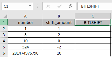
Here we have some values as number & shift_amount in Columns. We need to get the bitwise left shift operation on the given numbers using the BITLSHIFT function in excel

Use the formula :

=BITLSHIFT (A2, B2)

A2 : number provided to the function as cell reference
B2 : number provided to the function as cell reference

The bitwise left shift operation on 1 ( 01 ) by adding one zero to the right of the number will be 2 ( 010 ).

Now copy the formula to other cells using the Ctrl + D shortcut key.

As you can see here the BITLSHIFT function returns the result of the input values.

Notes:

Numbers can be given as argument to the function directly or using the cell reference in excel.
The numbers must be a valid decimal number between 0 & 281474976710655.
If a negative number is provided as Shift_amount argument to the function, the value shifts right.
The function returns the #NUM! Error
1. If either of the decimal number is less than 0 or greater than 281474976710655 which is 248-1.
2. If the resulting number exceeds the range of 0 to 248-1.
The function returns the #VALUE! Error,
1. If the input number is text or non-numeric.
2. If the shift_amount argument is text or non numeric.
3. If the shift amount is less than -53 or greater than + 53.

Hope you understood how to use BITLSHIFT function and referring cell in Excel. Explore more articles on Excel mathematical conversion functions here. Please feel free to state your query or feedback for the above article.