How to use the DOLLARDE function in Excel

In this article, we will learn How to use the DOLLARDE function in Excel.

Scenario :

What is fractional notation of a dollar price in decimals? Sometimes working with financial numbers, the existing dollar price in decimals needs to be converted to the special notation with the given fraction required.

New fractional notation = Integer price + decimal price (as integer) / fraction

Learn more about how to convert the dollar price to required dollar notation using the DOLLARDE function below.

How to use the DOLLARDE function

DOLLARDE function converts the dollar price (in decimal) to the type of fraction notation as per given fraction argument.

Generic formula:

=DOLLARDE (fractional_dollar, fraction)

fractional_dollar : dollar value in decimal

fraction : fractional value given as integer (denominator to the decimal part)

Example :

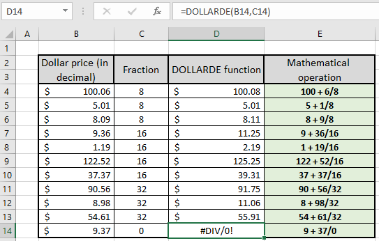
All of these might be confusing to understand. Let's understand this function using an example. Here we have a list of decimal values as fractional numbers and fractional part as Integer arguments.

Use the formula :

=DOLLARDE(B4,C4)

As you can see in the above image, the DOLLARDE function returns $100.08 which is also the mathematical expression of =100(int) + 06(decimal)/8(fraction). The mathematical expression in the right column can be used to understand the function in much better way. You can copy the formula to other cells using the Ctrl + D shortcut keys or dragging down from the right bottom of the D4 cell.

As you can see all the results obtained as per mathematical operation performed using the DOLLARDE function. As you inspect the D14 cell, there's a DIV! Error. It is generated as 37/0 returns non existing value i.e. in excel it is denoted by #DIV! Error.

Now let's see how different fractional values affect the same dollar price. For example we are considering $ 3.0625 as price.

As you can see in the example shown in the above image, how different fraction arguments affect the price value. Here the arguments to the function are given directly within the function.

You must be thinking why it is not possible to do the same task without using the function. It can be performed using the mathematical operation but there is a problem when you convert the decimal part of price to integer part.

Use the formula:

=INT(price)+(price-INT(price))*(10^n)/fraction

Here 10^n means if price value as upto 3 decimal place then n will be 3.

In the above example, we know that each price value has 2 digit decimal price so we used n = 2.

Here are some observational notes using the DOLLARDE function shown below.

Notes:

The formula only works with numbers.
Negative dollar price argument returns the dollar price with negative sign. But negative argument as fraction argument returns #NUM! error.
Blank cells are considered as zero value. Dollar price as 0 returns zero as result but zero as fraction argument returns #DIV! error.
The function returns #VALUE! Error if any argument to the function is non numeric.

Hope this article about How to use the DOLLARDE function in Excel is explanatory. Find more articles on mathematical operation and its related functions here. If you liked our blogs, share it with your friends on Facebook. And also you can follow us on Twitter and Facebook. We would love to hear from you, do let us know how we can improve, complement or innovate our work and make it better for you. Write to us at info@exceltip.com.

Related Articles :

How to use the DOLLAR function in Excel : Returns the number after rounding off the number upto specified decimal places using the DOLLAR function.

How to use the ROUND function in Excel : Rounds off the given number to the nearest num_digit decimal using the ROUND function in Excel

How to use the ROUNDUP function in Excel : Rounds up the given number to the nearest num_digit decimal using the ROUNDUP function in Excel.

How to use the ROUNDDOWN function in Excel : Rounds down the given number to the nearest num_digit decimal using the ROUNDDOWN function in Excel.

How to use the FLOOR.MATH function in Excel : Rounds down the number to the nearest specified multiple using the FLOOR.MATH function in Excel.

How to use the MROUND function in Excel : rounds off the number to the nearest specified multiple using the MROUND function in Excel.

Popular Articles:

How to use the IF Function in Excel : The IF statement in Excel checks the condition and returns a specific value if the condition is TRUE or returns another specific value if FALSE.

How to use the VLOOKUP Function in Excel : This is one of the most used and popular functions of excel that is used to lookup value from different ranges and sheets.

How to Use SUMIF Function in Excel : This is another dashboard essential function. This helps you sum up values on specific conditions.

How to use the COUNTIF Function in Excel : Count values with conditions using this amazing function. You don't need to filter your data to count specific values. Countif function is essential to prepare your dashboard.