The Excel MAXIFS Function

The Excel MAXIFS function is a new function, introduced in Excel 365 and 2019. This function returns the MAX value from a given range.
In this article, we will learn how to use the MAXIFS function in Excel.

Syntax of MAXIFS Function

=MAXIFS(max_range,criteria_range1,criteria1,...)

Max_range1: It is the numeric range that contains the max value.
Criteria_range1: It is the criteria range that you want to filter before getting max value.
Criteria1: It is the criteria or the filter that you want to put on criteria_range before getting the Max value.

You can have multiple pairs of criteria_range and criteria.

Let’s understand the MAXIFS function with an example.

Example of MAXIFS Function
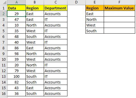
So, here I have a table of some data. The first column contains the numeric values. Second column contains the Region and the third column has the department.

The task is to tell the max value from the first range for each region.

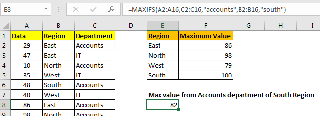
The formula for getting maximum value from "East" region will be:

=MAXIFS(A2:A16,B2:B16,"East")

It will return 82.
Here we have given hardcoded criteria, but we can also give reference of the criteria to make it dynamic.

=MAXIFS($A$2:$A$16,$B$2:$B$16,E2)

Here we have used absolute ranges to lock the max range and criteria range.

You can put more than 1 criteria in MAXIFS function. For example, if I want to get MAX value from IT department of SOUTH region then the formula will be:

=MAXIFS(A2:A16,C2:C16,"IT",B2:B16,"SOUTH")

This will return 100 as per above data. If we put "Accounts" in place of IT, the MAXIFS will return 82.

So yeah guys, this was a small introduction to the MAXIFS function of Excel 365 and 2019. I hope it was helpful. If you have any doubts regarding this article or any other excel topic, ask in the comments section below.

Related Article

Calculate Max if condition match | To calculate the MAX value with a condition in Excel 2016 and older versions, use this formula. Using the MAX and IF function together we can get a conditional Max output.

Excel 2019/365 Functions:

How to Use The Excel UNIQUE Function | The UNIQUE function returns the Unique values from the given array.

The SORT Function in Excel | The SORT function returns the sorted form of the supplied array.

How to Use Excel SORTBY Function | The SORTBY function sorts a given range by a different specified range. Sorting range does not need to be part of the table.

How to Use The Excel FILTER Function | The FILTER function returns all matched values of given criteria and spills the result into adjacent cells.

The SEQUENCE Function in Excel | The SEQUENCE function returns a series of sequential numbers. It is a dynamic array formula.

Popular Articles:

50 Excel Shortcuts to Increase Your Productivity | Get faster at your task. These 50 shortcuts will make you work even faster on Excel.

How to use the VLOOKUP Function in Excel | This is one of the most used and popular functions of excel that is used to lookup value from different ranges and sheets.

How to use the COUNTIF function in Excel 2016 | Count values with conditions using this amazing function. You don't need to filter your data to count specific values. Countif function is essential to prepare your dashboard.

How to use the SUMIF Function in Excel | This is another dashboard essential function. This helps you sum up values on specific conditions.