
In this article, we will learn How to use the FVSCHEDULE function in Excel.
Scenario:
In financial terms, when lending or borrowing money having various compound interest rates. For example, having a loan agreement with an initial investment and having different interest rates for different compounding years. FV function returns the future value considering the same interest rate for the whole period. It can't have multiple interest rates in the same formula Let's understand FVSCHEDULE function arguments explained below
FVSCHEDULE function in Excel
FVSCHEDULE function takes present value or initial principal amount and interest rates for different periods are given as schedule array in argument.
FVSCHEDULE function syntax:
| =FVSCHEDULE (principal, schedule) |
principal : initial amount or present value at the start of first year
schedule : scheduled interest rates given as an array.
Example :
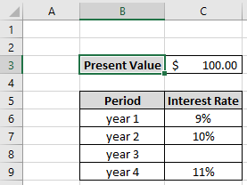
All of these might be confusing to understand. Let's understand this function using an example. For example, Mr Trump has borrowed 100 dollars with terms having condition that if he is not able to pay the initial principal amount with interest rate, the interest rate will increase by 1 percent for each year (3rd year is exception)
Use the formula:
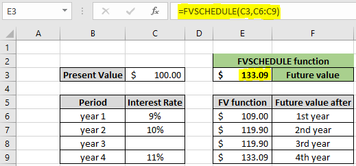
| =FVSCHEDULE(C3,C6:C9) |
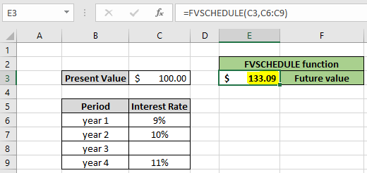
As you can see in the image shown above, the function returns $ 133.09 as future value i.e Mr trump will pay $133.09 at the end of 4th year. The function takes blank cells as 0% for the corresponding year. You must be thinking is it possible to calculate the future value using the FV function. Let's understand how to perform FV function with different interest rates.
FV function with different interest rates for different year period
For the same example shown above, we will calculate the future value using the FV function. But for different interest rates we will use different formulas.
Use the formula for 1st year
| =FV(C6,1,0,-C3) |
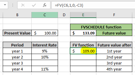
As you can see, Mr Trump will return $ 109.00 at the end of first period, if not then present value for the second year will be $ 109.00
Use the formula for 2nd year
| =FV(C7,1,0,-E6) |
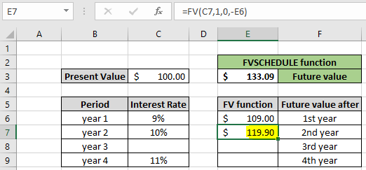
Mr Trump will have to $ 119.90 at the end of second year. Similarly calculating for each year will returns the same amount as the FVSCHEDULE function at the end of 4th year.
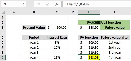
As you can see now the formula at the end of 4th year returns $ 133.09 i.e. Mr Trump is in a lot of debt till the 4th year. When calculating for the 20 years with different interest rates, we can't use the FV function, but the FVSCHEDULE function is quite handy for these kinds of problems.
Here are some observational notes using the FVSCHEDULE function shown below.
Notes :
Hope this article about How to use the FVSCHEDULE function in Excel is explanatory. Find more articles on financial formulas and related functions here. If you liked our blogs, share it with your friends on Facebook. And also you can follow us on Twitter and Facebook. We would love to hear from you, do let us know how we can improve, complement or innovate our work and make it better for you. Write to us at info@exceltip.com.
Related Articles
How to use the PV function in Excel : The PV function returns the present value of investment for the expected future value with given interest rate and time period in Excel. Learn more about PV function here.
How to use the FV function in Excel : The FV function returns the future value of investment for the present value invested with a given interest rate and time period in Excel. Learn more about the FV function here.
Excel PV vs FV function : find Present Value using PV function and future value using FV function in Excel.
How to use the RECEIVED function in excel : calculates the amount which is received at maturity for a bond with an initial investment (security) and a discount rate, there are no periodic interest payments using the RECEIVED function in excel.
How to use the NPER function in excel : NPER function to calculate periods on payments in Excel.
How to use the PRICE function in excel : returns the price per $100 face value of a security that pays periodic interest using the PRICE function in Excel.
Popular Articles:
How to use the IF Function in Excel : The IF statement in Excel checks the condition and returns a specific value if the condition is TRUE or returns another specific value if FALSE.
How to use the VLOOKUP Function in Exceln : This is one of the most used and popular functions of excel that is used to lookup value from different ranges and sheets.
How to Use SUMIF Function in Excel : This is another dashboard essential function. This helps you sum up values on specific conditions.
How to use the COUNTIF Function in Excel : Count values with conditions using this amazing function. You don't need to filter your data to count specific values. Countif function is essential to prepare your dashboard.
The applications/code on this site are distributed as is and without warranties or liability. In no event shall the owner of the copyrights, or the authors of the applications/code be liable for any loss of profit, any problems or any damage resulting from the use or evaluation of the applications/code.


