How to use the INDIRECT function in Excel

In this article, we will learn about how to use the INDIRECT function in Excel.

For what in Excel INDIRECT function in used

Cell reference and array reference is the most common usage for an excel user. It means picking up the value using the cell address so as to just change the value in the cell to get the new result. For example if you need to find the sum of the first 20 numbers in column A, you would use =SUM(A1:A120) . Now if you need for next 20. You have to edit the whole formula. Now you know the INDIRECT function which will help you understand the efficient use excel formula.

INDIRECT function in Excel

The INDIRECT function is a cell reference function. It takes the value in the cell as address and returns the value in the address cell.

INDIRECT function Syntax:

=INDIRECT (ref_text, [a1])

Problem 1

Let’s understand this function using it in an example.

Here As you can see B1 has the Formula indicating A1 cell and Text in A1 is D1. So the function returns the value in the D1 cell which is 500.

You can use it in many forms as shown here

Here & operator is used for joining the text to get a full address of the cell. So A1 has D and 1 is added to D, get D1 cell ref.

You can directly refer to any cell.

Here D1 is directly supplied to get the return from D1 address.

SUM values in range using INDIRECT function

You can use it with other functions to get the sum of the range given by cell reference.

Here Range is provided to Sum functions referring A2:A5 cell. Let's understand more about from another problem.

How to solve the problem?

For this problem, we will be considering the way we use to pick elements from the same sheet, then we will use the formula to extract a list of values from different sheets. Excel INDIRECT & CELL function will be used to make a formula to do so as explained below.

Generic formula:

=INDIRECT ( "sheet_name" & "!" & CELL( "address", cell_ref)

sheet_name : sheet name

cell_ref : cell reference without sheet name.

Example :

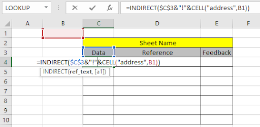
All of these might be confusing to understand. Let's take an example to understand how to use the formula to extract an array of values from the different sheets. Here we have a worksheet having values in different sheets. We need to extract a list of values using the formula

Use the formula:

=INDIRECT ( $C$3 & "!" & CELL("address",B1))

Explanation:

When extracting a value from the different sheet. The excel accepts a syntax which is Sheet1!B1. (Here Sheet1 is sheet name and B1 is cell reference).
The CELL function returns the cell reference and feeds the reference to the INDIRECT function.
& operator joins or concatenates the two or more arguments.
INDIRECT function returns the value in the cell reference provided.

Here B1 is a cell reference of the same sheet but value is extracted from the Data sheet.

The value in the Data sheet B1 cell is 5800. Copy the formula to get the list of values starting from the value extracted from the first result.

Here we have the list of values starting from the B1 to B7 cell of the Data sheet.

Excel increment cell reference from different sheet using cell reference.

We know how to get cell reference increment from the same sheet. Let's use a formula to extract value from the same sheet. Generic Formula is =cell_ref.

What this formula does is paste picks the value from the address which is the cell reference. When a cell reference is used within a formula. It can be used for various tasks and value gets updates as value gets updated from the cell. Extend the formula to below cells to get a list of values.

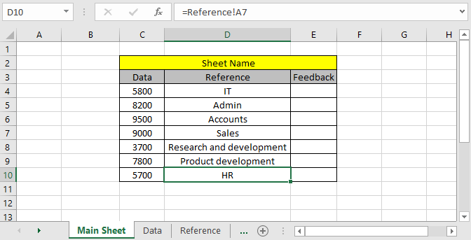
As you can see here we have the required arrey. Now we need to get these values to the main sheet. Excel accepts the syntax when extracting values from different sheet which is =Reference!A1. (Here Reference is sheet name and A1 is cell reference).

Copy the formula to the remaining cells using the Ctrl + D or drag down from the right bottom of the cell.

As you can see, here we have all the required values from the Reference sheet. There's one more method to get the values from different sheets.

Extract list of values from different sheets using named range.

We can use a method to call the whole array directly using the named range from different sheets. For this, we will just select the array or table and name the selected part in the name box and call it by the name wherever required in the worksheet.

Here selected the whole table and named it Data. Name box is found on the top left corner of the sheet as highlighted in the above sheet.

We will extract the named table in the new sheet. Go to the new sheet and select the same number of cells and type the formula stated below.

Use the formula:

{ =Data }

Note : use Ctrl + Shift + Enter instead of Enter to the formula working for arrays. Do not use put curly braces manually.

As we can see the formula works fine. Any of these methods can be used wherever needed.

Here are all the observational notes regarding using the formula.

Notes:

These formulas only extract values not the format. You can apply the same formatting using the format painter tool across sheets.
Value gets updated as we change the value in cell reference.
We can edit the values inside the formula using different operators like mathematical operator for numbers, "&" operator for text values.

Hope this article about How to use the INDIRECT function in Excel is explanatory. Find more articles on calculating values and related Excel formulas here. If you liked our blogs, share it with your friends on Facebook. And also you can follow us on Twitter and Facebook. We would love to hear from you, do let us know how we can improve, complement or innovate our work and make it better for you. Write to us at info@exceltip.com.

Related Articles :

All About Excel Named Ranges : excel ranges that are tagged with names are easy to use in excel formulas. Learn all about it here.

The Name Box in Excel : Excel Name Box is nothing but a small display area on top left of excel sheet that shows the name of active cell or ranges in excel. You can rename a cell or array for references.

How to Get Sheet name of worksheet in Excel : CELL Function in Excel gets you the information regarding any worksheet like col, contents, filename, ..etc. Learn how to get the sheet name using the CELL function here.

How To Get Sequential Row Number in Excel : Sometimes we need to get a sequential row number in a table, it can be for a serial number or anything else. In this article, we will learn how to number rows in excel from the start of data.

Increment a number in a text string in excel : If you have a large list of items and you need to increase the last number of the text of the old text in excel, you will need help from the two TEXT and RIGHT functions.

Popular Articles :

How to use the IF Function in Excel : The IF statement in Excel checks the condition and returns a specific value if the condition is TRUE or returns another specific value if FALSE.

How to use the VLOOKUP Function in Excel : This is one of the most used and popular functions of excel that is used to lookup value from different ranges and sheets.

How to use the SUMIF Function in Excel : This is another dashboard essential function. This helps you sum up values on specific conditions.

How to use the COUNTIF Function in Excel : Count values with conditions using this amazing function. You don't need to filter your data to count specific values. Countif function is essential to prepare your dashboard.