In this article, we will learn about the ISERR function in Excel.
ISERR is a built-in Excel logical function. It’s a Logical function which checks the condition and returns TRUE if there’s any error like #VALUE!, #REF!, #DIV/0!, #NUM!, #NAME?, or #NULL! Except #N/A and otherwise.
The ISERR function is used with other logic functions like IF function to help with calculations. The IF function perform mathematical operations on the data value and sometimes in return it generates error like #VALUE!, #REF!, #DIV/0!, #NUM!, #NAME?, or #NULL!. So to get the error free results in the table, use the ISERR function.
ISERR checks for various errors in any condition like #VALUE!, #REF!, #DIV/0!, #NUM!, #NAME?, or #NULL! returns TRUE and returns FALSE for #N/A error and otherwise.
Syntax:
value : value to the function can be provided as cell reference or directly.
Now let’s understand the function more via using it in an example
1st error is division error denoted by #DIV/0!. This is generated when any number is divided by the number zero.

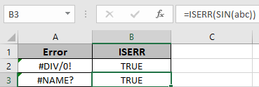
Use the ISERR function as shown in the snapshot above to return Logic value like TRUE or FALSE except the division error.
2nd error is name error denoted by #NAME? . This is generated when excel doesn’t understand the input argument. Here we provide text to the SIN function without using quotes, the function returns the #NAME? error.

Use the ISERR function as shown in the snapshot above to return Logic value except showing the error.
3rd error is Not Applicable error denoted by #NA! . This is generated when the formula doesn’t find the match value, so its show no value available error. Here the value to the function is provided as cell reference.

The function returns FALSE, as the function returns TRUE for all errors except #NA! error.
Use the ISERR function as shown in the snapshot above to return Logic value except showing the error.
4th error is reference error denoted by #REF! . This is generated when the reference to the function is invalid cell.

Use the ISERR function as shown in the snapshot above to return Logic value like TRUE or FALSE except showing the error.
5th error is num error error denoted by #NUM! . This is generated when

Use the ISERR function as shown in the snapshot above to return Logic value like TRUE or FALSE except showing the error.
6th error is VALUE error denoted by #VALUE! . This is generated when the input argument to the function is wrong.

Use the ISERR function as shown in the snapshot above to return Logic value except showing the error.
7th error is null error denoted by #NULL! . This is generated when the operation to the arguments of the function is absent or invalid.
Here the #NULL! Error is generated using the space between the two referred cells and due to absence of operation between the two returns the #NULL! error.

Use the ISERR function as shown in the snapshot below to return Logic value except showing the error.

As you can see the function returns the logic values either TRUE or FALSE. Catch these errors using the ISERR function and return the values instead of the errors.
Hope you learnt about how to use ISERR function in Excel 2016. Find more articles on Excel error function like ISERROR and NA function here. Please share your query below in the comment box. We will assist you.
Related Articles
How to use the ISERROR function in Excel
How to use the ISNA function in Excel
How to use the IFNA function in Excel
How to use the NA function in Excel
Popular Articles
Edit a dropdown list
If with conditional formatting
If with wildcards
Vlookup by date
The applications/code on this site are distributed as is and without warranties or liability. In no event shall the owner of the copyrights, or the authors of the applications/code be liable for any loss of profit, any problems or any damage resulting from the use or evaluation of the applications/code.