How to use the ISNUMBER function in Excel

In this article, we will learn How to use the ISNUMBER function in Excel.

Number or text or boolean in Excel

There are Four types of input value in Excel. First is a number like date, time, currency or percentage. Second is boolean which can be 1 or 0 and can be interpreted as TRUE (1) or FALSE (0). Third is error value like #DIV/0! Error. All the rest comes under text value mostly with space characters and alphabets like "1 0" is 1 and 0 with a space between them, so "1 0" will be considered as text value. Excel provides you with some functions which let you check the type of value in a cell. One of these functions is ISNUMBER function, This function is mostly used with functions which return numbers or errors like the FIND function. Let's learn more about ISNUMBER function syntax and an example to illustrate the function usage.

ISNUMBER Function in Excel

Excel’s ISNUMBER function is a boolean function that returns TRUE or FALSE, if supplied value is a number or non-number, respectively.

ISNUMBER Function Syntax :

=ISNUMBER (cell_ref)

cell_ref : cell reference of cell to check. e.g. =ISNUMBER(B2)

It simply takes one argument and returns TRUE if its a number else FALSE. Most of the time you will pass references of a cell or a formula as values to check if it's a number or not.

Example :

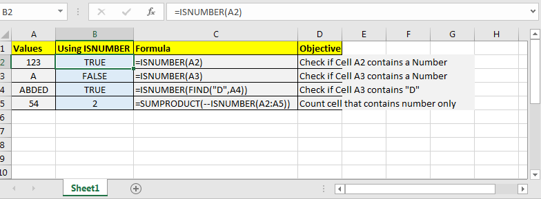
All of these might be confusing to understand. Let's understand how to use the function using an example. Here we have some values to show the functionality of the ISNUMBER function.

Check if Cell A2 contains a number or not

=ISNUMBER(A2)

Check If formula returns a number or not

=ISNUMBER(FIND(“A”,A2))

Count cells that contain numbers.

You can pass the whole range to ISNUMBER function. It will show if only the first element is a number or not but internally it will store an array of true and false. It comes in handy while working with excel formulas that accept arrays as input.

=SUMPRODUCT(--(ISNUMBER(A2:A10)))

As you can see the extracted results using the ISNUMBER function.

ISNUMBER with other functions like FIND :

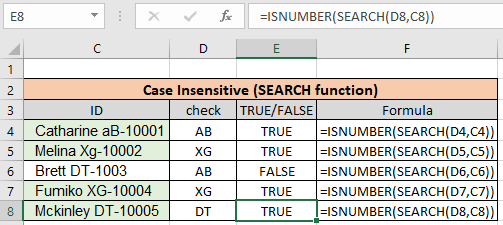
The below example is great usage to check the results returned by FIND function converted to TRUE or FALSE. Let's understand how to use the function using an example. Here we have some employees to look up by the given department Id. Employee id has name, department id and particular id. Here lookup text is in column D and within text is in Column C.

Use the formula:

=ISNUMBER(SEARCH(D4,C4))

As you can see the formula finds aB when you looked for

AB using the Search function. Copy the formula to the rest of the cells using the Ctrl + D or dragging it down from the right bottom (tiny box) of the applied cell.

As you can see we found all the given department id employees using the above method. Now we will check if all cells contain specific text.

Another Example: (Case Sensitive)

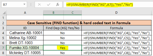
Here we have been given a list of Employee Id information in column A and the look up department is "XG". Here we need to find the department "XG" in all cells. "XG" must be exact as there are two different departments that go by "Xg". So check only "XG" in all cells and return "Yes" if found and return "No" If not.

Use the formula:

=ISNUMBER(FIND(D4,C4))

As you can see First employee doesn't belong to "XG" so the formula returns "No" using the FIND function. Copy the formula to the rest of the cells using the Ctrl + D or dragging it down from the right bottom (tiny box) of the applied cell.

As you can see there is only one employee in "XG" department. This formula is useful wherever the database contains multiple information of a row in one cell.

Here are all the observational notes using the ISNUMBER function in Excel
Notes :

The function returns TRUE only if any number is given as input. It returns FALSE for boolean values (TRUE and FALSE). To check boolean values in a list use the ISLOGICAL function in Excel. Use ISTEXT function to check text in cell
There are more functions to check numbers like ISODD function and ISEVEN function.

Hope this article about How to use the ISNUMBER function in Excel is explanatory. Find more articles on checking values and related Excel formulas here. If you liked our blogs, share it with your friends on Facebook. And also you can follow us on Twitter and Facebook. We would love to hear from you, do let us know how we can improve, complement or innovate our work and make it better for you. Write to us at info@exceltip.com.

Related Articles :

How to use the ISEVEN function in Excel : returns the TRUE logic value if the number is even using the ISEVEN function in Excel.

How to use the ISODD function in Excel : returns the TRUE logic value if the number is ODD using the ISODD function in Excel.

How to use the ISERROR function in Excel : returns the TRUE logic value if the cell value is error using the ISERROR function in Excel.

How to use the ISTEXT function in Excel : returns the TRUE logic value if the cell value is text using the ISTEXT function in Excel.

How to use nested IF function : nested IF function operates on data having multiple criteria. The use of repeated IF function is nested IF excel formula.

Using the IF with AND / OR Functions in Microsoft Excel : These logical functions are used to carry out multiple criteria calculations. With IF the OR and AND functions are used to include or exclude matches.

Popular Articles :

How to use the IF Function in Excel : The IF statement in Excel checks the condition and returns a specific value if the condition is TRUE or returns another specific value if FALSE.

How to use the VLOOKUP Function in Excel : This is one of the most used and popular functions of excel that is used to lookup value from different ranges and sheets.

How to use the SUMIF Function in Excel : This is another dashboard essential function. This helps you sum up values on specific conditions.

How to use the COUNTIF Function in Excel : Count values with conditions using this amazing function. You don't need to filter your data to count specific values. Countif function is essential to prepare your dashboard.