In this article, we will learn How to use the MID function in Excel.
What do LEFT, MID & RIGHT functions do in Excel ?
LEFT function returns the part of word from the start of word.
"abcdefg" extracting 3 from start returns "abc"
RIGHT function returns the part of word from the ending of word.
"abcdefg" extracting 3 from end returns " efg"
MID function returns the part of word from given starting point till number of counts given.
"abcdefg" extracting 3 from the 2nd position returns "bcd".
You can use the MID function as a LEFT function or RIGHT function just changing the start point. But vice versa is not possible.
MID Function in Excel
MID function returns the part of a given word. The Excel MID function is used to extract text from mid of a string. Basically n number of characters from a given index in string.
MID function syntax :
| =MID(text, start_num, num_of_chars) |
text : text or word to extract from
start_num : starting point number or starting position
num_of_chars : n number of characters to pick.
Example :
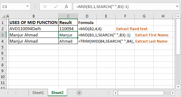
All of these might be confusing to understand. Let's understand how to use the function using an example. Here given the word "AVD110094Delhi". We need to extract the 6 digit code in between the word which starts from 4th position.
If you know from which position how many characters are needed to extract simply use MID function. The below formula will extract city code 110094.
Use the formula in C2 cell (Extract fixed text)
| =MID(“AVD110094Delhi”,4,6) |

Here text is “AVD110094Delhi”.
Start_num is 4 since city code starts from 4th position.
Num_of_chars is 6 because city code is 6 characters long.
Here we knew how many characters there were and from which position they started. What if we don’t know this? Next example illustrates another amazing use of the MID function.
Extract First Name Using Excel MID Function
Generic Formula to Extract First Name in Excel 2016
| =MID(text,1,SEARCH(“ “,text)-1) |
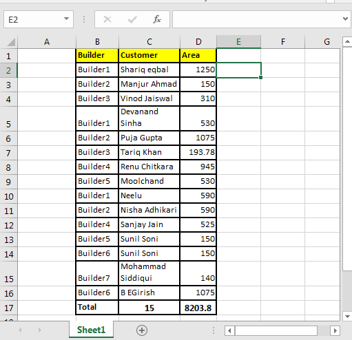
I have this table. Now, I want to extract my first name from column C.
To extract first name write this MID formula and drag it down:
| =MID(C2,1,SEARCH(" ",C2)-1) |
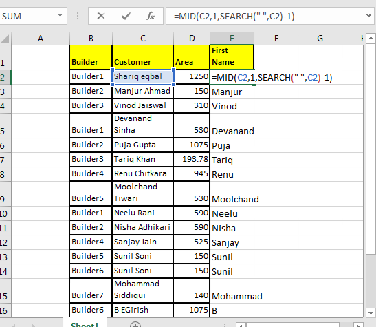
Here, we knew the starting point (start_num) for first name but didn’t knew the number of characters in first name.
So we took SEARCH function’s help to find the “space” (“ ”) in text.
Then we subtracted 1 to exclude that space from extracted text. Simple.
Extract Last Name Using Excel MID Function
Generic Formula to Extract Last Name in Excel 2016
| =TRIM(MID(C2,SEARCH(" ",C2),LEN(B2))) |
In the same table write this formula…
| =TRIM(MID(C2,SEARCH(" ",C2),LEN(B2))) |
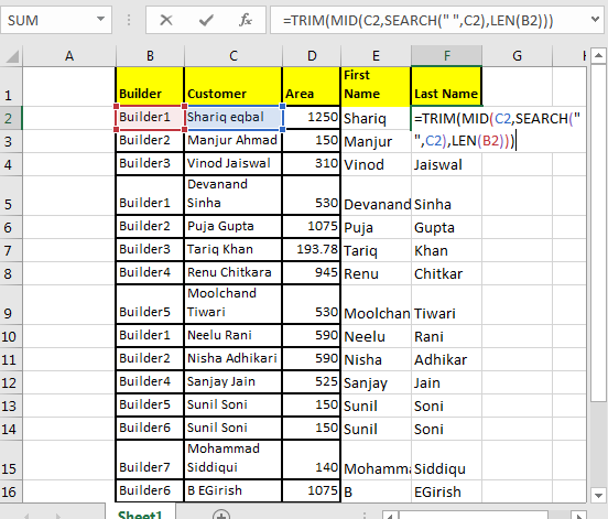
Here we don’t know the start_num nor the num_chars.
To find the start_num we took help from the SEARCH function.
We don’t know the number of characters to extract. And we don’t need to. We will just use the LEN function. It will give the length of the string. Hence it will return all the characters remaining after start_num.
Each column should contain only one kind of value. Once it’s done we can make pivot reports in excel that will tell us better about the data. So let's learn about LEFT function and RIGHT function in Excel.
Extract Text From A String In Excel Using Excel’s LEFT And RIGHT Function
I have received data that looked like garbage, but using excel RIGHT and LEFT functions I have turned them into meaningful reports. Data cleaning in excel is easy. Here I am going to explain how you can extract specific text in excel 2016 from a cell and leave behind garbage data.

In the above image, I am provided with data in Excel. It has Name, Age, and if the person has any insurance or no (Y/N). To use this data, I need to extract data in different columns.
Excel RIGHT Function to Extract Data From Right of The Text

The RIGHT function in excel takes only two arguments. First the TEXT, and second the NUMBER OF CHARACTERS you want to extract from the right in excel.
Here, we have our text in cell B3 and the number of characters we want to extract is 1. Just write this formula in excel in cell D3 or wherever you want to have this data.
| =RIGHT(B3,1) |
You will have your result in cell D3. just copy or drag down this formula in the cells below.
Excel LEFT Function to Extract Data From Left of The Text
Now let's get our age. Before explaining, let me show you the formula. Copy this formula in desired cells.
Use the formula :
| =LEFT(RIGHT(B3,4),2) |
In the above formula, we have combined LEFT and RIGHT functions to get our specific text from the string. This is how it looks.
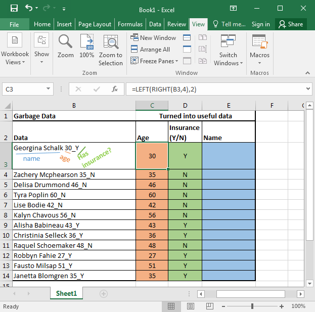
Every function works from inwards to outwards. So let's start with:
RIGHT(B3,4): It simply extracts 4 characters from a given text. That gives us 30_Y. Why 4? Since we know that age is only one of two characters, and we have 1 “_” and 1 Y or N.
LEFT(RIGHT(B3,4),2): Now we have our text that starts with age that is of 2 characters. Here comes the LEFT function into action. It takes RIGHT(B3,4) as its text argument and extracts 2 characters from that. That gives us 30 for the first cell. Copy the formula in the cells below and you will get the rest of the data as shown in the image above.
Just like the RIGHT function, LEFT function also takes two same arguments. It just extracts data from the left of the string provided.
Excel LEFT and Right Function to Extract unknown length of Text from a String
Just paste this formula in desired cells to extract the name from the text in excel.
| =LEFT(B3,LEN(B3)-5) |
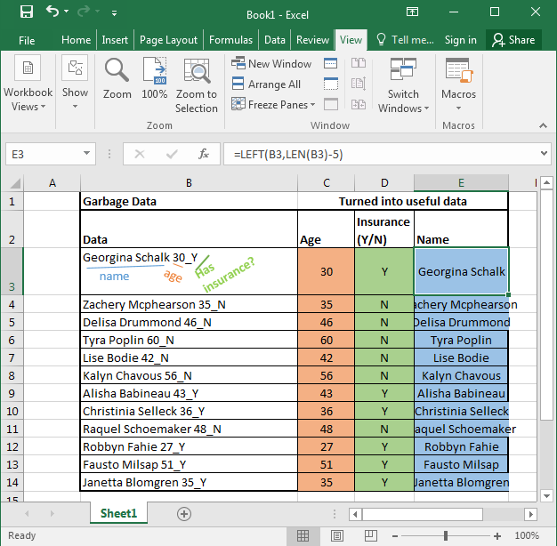
In the above examples, we knew the exact number of texts to extract from the given text.
Hope this article about How to use the MID function in Excel is explanatory. Find more articles on calculating values and related Excel formulas here. If you liked our blogs, share it with your friends on Facebook. And also you can follow us on Twitter and Facebook. We would love to hear from you, do let us know how we can improve, complement or innovate our work and make it better for you. Write to us at info@exceltip.com.
Related Articles :
Searching a String for a Specific Substring in Excel : Find cells if cell contains given word in Excel using the FIND or SEARCH function.
Highlight cells that contain specific text : Highlight cells if cell contains given word in Excel using the formula under Conditional formatting
How to Check if a string contains one of many texts in Excel : lookup cells if cell contains from given multiple words in Excel using the FIND or SEARCH function.
Count Cells that contain specific text : Count number of cells if cell contains given text using one formula in Excel.
How to lookup cells having certain text and returns the Certain Text in Excel : find cells if cell contains certain text and returns required results using the IF function in Excel.
Popular Articles :
How to use the IF Function in Excel : The IF statement in Excel checks the condition and returns a specific value if the condition is TRUE or returns another specific value if FALSE.
How to use the VLOOKUP Function in Excel : This is one of the most used and popular functions of excel that is used to lookup value from different ranges and sheets.
How to use the SUMIF Function in Excel : This is another dashboard essential function. This helps you sum up values on specific conditions.
How to use the COUNTIF Function in Excel : Count values with conditions using this amazing function. You don't need to filter your data to count specific values. Countif function is essential to prepare your dashboard.
The applications/code on this site are distributed as is and without warranties or liability. In no event shall the owner of the copyrights, or the authors of the applications/code be liable for any loss of profit, any problems or any damage resulting from the use or evaluation of the applications/code.