How to use the MIRR function in Excel

In this article, we will learn about how to use the MIRR function in Excel.

MIRR function returns the Modified interest rate of return for the financial data having Investment, finance rate & reinvestment_rate.

The MIRR function returns modified interest rate of return in percentage.
Syntax:

=MIRR (values, finance_rate, reinvest_rate)

Values : Investment amount (both positive & negative amount) or cash flows in array.
Finance_rate : Required rate of return (discount rate) as a percentage.
Reinvest_rate : Interest rate received on cash flows reinvested as percentage.

Let’s understand this function using it in an example.

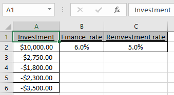
Here we have Investment, Finance_rate & reinvestment_rate.

Investment or cash flow array must contain both positive & negative amounts.

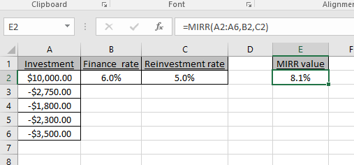
Use the formula:

=MIRR(A2:A6, B2, C2)

A2:A6 : investment amount or cash flow
B2 : finance_rate
C2 : Reinvest_rate

As you can see the MIRR function returns the modified interest rate of return is 8.1%.
Hope you understood how to use the MIRR function to get modified interest rate of return in Excel. Explore more articles on Excel financial functions here. Please feel free to state your query or feedback for the above article.