In this article, we will learn How to use the OFFSET function in Excel.
What is OFFSET Function?
Offset function is an information retrieval function. If you have a huge table containing certain data and you want to retrieve data from it, the best way to do it is insert an offset formula for the table in that worksheet or another sheet in the same workbook. Thus, once you have created the offset retrieval table, you simply have to enter the data for example ‘month’ and you will get the ‘sales’ or ‘income’ of that month from that table.
Going through the table is another option, but would you consider the option if you have sheets and sheets of data all containing a 1000 column data table? This is where offset is combined with other functions.
The concept of pivot table comes from offset. A pivot table is a general table and from that specific combination of data and graphs is obtained as and when required. Also dynamic tables can be created in the same manner. For these tables you will have to create the excel offset formula
Syntax of OFFSET
| =OFFSET(reference,rows, columns, [height], [width]) |
Rows – you ask excel to move the number of rows to get the info. In this case it has to move all around the table and so simply leave a blank denoted by a comma (,). Otherwise, to move a column forward give value as 1 and to move a column prior give a value -1.
Columns – this is to drive the function to the number of columns. The value system is same as that for row.
Height – the height of the table, in this case A11.
Width – width of the table, in this case D11.
After you set up the offset function, running a trial is important to weed out any errors.
Let us take a table that contains Name, email id, date of birth and age. The table begins at A1 cell, containing the ‘Name’ heading. The data runs for say A11. And the rows run till D1. The entire table runs A1:D11. You want a retrieval system that gets you the name when you enter the email id, or the email id when you enter the name along with other details. You create a formula by satisfying the 5 arguments.
Reference point is the cell from which the look up should start. In this case it should be A2. That is the general standard.
Example:
For example you give reference of B4 and offset row 0, and offset column 1 then value from C4 will be returned. Confusing? Lets have some more examples. Last example of OFFSET function tells how to SUM dynamically.
OFFSET Function to Get value From Right and Left of a Cell
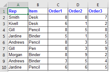
We have this table.

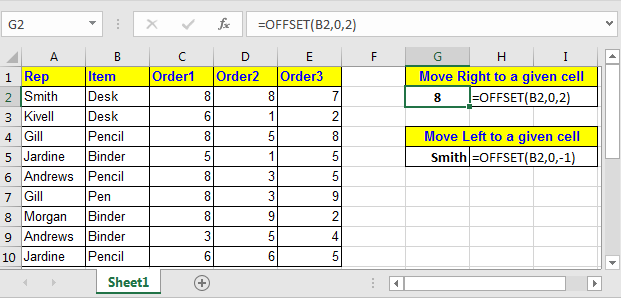
Now if I want to get value from 2 cell right to B2 (which means D2). I will write this OFFSET formula:
| =OFFSET(B2,0,2) |
OFFSET function will move 2 cell to right of cell B4 and return its value. See Image below
If I want to get value from 1 cell left to B2 (which means A2). I will write this OFFSET formula:
| =OFFSET(B2,0,-1) |
Minus (-) sign indicates offset to move reversed.

OFFSET Function to Get value From Below and Above of a Cell
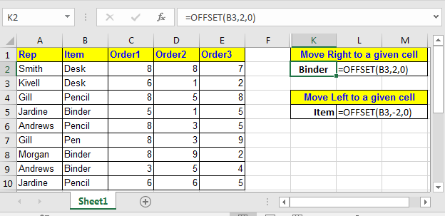
So again in the above table, if I want to get value from 2 cell belove to B3 (which means B5). I will write this OFFSET formula:
| =OFFSET(B2,2,0) |
If I want to get value from 1 cell left to B2 (which means A2). I will write this OFFSET formula:
| =OFFSET(B2,-2,0) |

OFFSET Function to Sum Range Dynamically
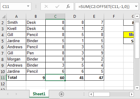
Lets see this example.

In above table Total row in end of table. Over the time you will add rows to this table. Then you’ll need to change sum range in formula. Here we can take help of OFFSET function to sum dynamically. Currently in cell C11 we have =SUM(C2:C10). Replace this with below formula.
| =SUM(C2:OFFSET(C11,-1,0)) |
This formula just takes the first data row and then sums the range above the total row.

Offset For Getting Array
OFFSET function has two optional arguments, [height] and [width]. Do not take them for granted. When OFFSET function is provided [height] and [width] arguments, it returns a two dimensional array. If only one of them is passed as argument it returns on dimensional array of values.
If you type in this formula in any cell :
| =SUM(OFFSET(C1,1,0,9,3)) |
It will sum values in range starting from C2 to 9 rows below and 3 columns right.
OFFSET(C1,1,0,9,3) : This will translate to {8,8,7;6,1,2;8,5,8;5,1,5;8,3,5;8,3,9;8,9,2;3,5,4;6,6,5}.

So in conclusion, offset is very useful function of excel that can help you solve many strangled threads. Let me know how you use OFFSET function in your formula and where it helped you most.
Lookup function is same as offset but utilizes functions such as Match, Counta and IF to work a dynamic table.
Using offset in Excel requires skill and good knowledge of Excels functions and how they work together. Pulling it off without any error is the biggest hurdle.
Here are all the observational notes regarding using the formula.
Notes:
Hope you understood What is Excel Offset Function and How to Use it in Excel. Explore more articles on Excel lookup and match values using formulas here. If you liked our blogs, share it with your friends on Facebook. And also you can follow us on Twitter and Facebook. We would love to hear from you, do let us know how we can improve, complement or innovate our work and make it better for you. Write to us at info@exceltip.com.
Related Articles
VLOOKUP function to calculate grade in Excel : To calculate grades IF and IFS are not the only functions that you can use. The VLOOKUP is more efficient and dynamic for such conditional calculations.To calculate grades using VLOOKUP we can use this formula.
17 Things About Excel VLOOKUP : VLOOKUP is most commonly used for retrieving matched values but VLOOKUP can do a lot more than this. Here are 17 things about VLOOKUP that you should know to use effectively.
LOOKUP the First Text from a List in Excel : The VLOOKUP function works fine with wildcard characters. We can use this to extract the first text value from a given list in excel. Here is the generic formula.
LOOKUP date with last value in list : To retrieve the date that contains the last value we use the LOOKUP function. This function checks for the cell that contains the last value in a vector and then uses that reference to return the date.
How to Retrieve Latest Price in Excel : It is common to update prices in any business and using the latest prices for any purchase or sales is must. To retrieve the latest price from a list in Excel we use the LOOKUP function. The LOOKUP function fetches the latest price.
Popular Articles:
50 Excel Shortcut to Increase Your Productivity : Get faster at your task. These 50 shortcuts will make you work even faster on Excel.
How to use the IF Function in Excel : The IF statement in Excel checks the condition and returns a specific value if the condition is TRUE or returns another specific value if FALSE.
How to use the VLOOKUP Function in Excel : This is one of the most used and popular functions of excel that is used to lookup value from different ranges and sheets.
How to use the COUNTIF Function in Excel : Count values with conditions using this amazing function. You don't need to filter your data to count specific values. Countif function is essential to prepare your dashboard.
How to use the SUMIF Function in Excel : This is another dashboard essential function. This helps you sum up values on specific conditions.
The applications/code on this site are distributed as is and without warranties or liability. In no event shall the owner of the copyrights, or the authors of the applications/code be liable for any loss of profit, any problems or any damage resulting from the use or evaluation of the applications/code.